

About Corridor Design
The Corridor Designer Tools port and modernize CorridorDesigner — the wildlife-linkage design toolkit developed by Paul Beier, Dan Majka and Jeff Jenness at Northern Arizona University (corridordesign.org) — for ArcGIS Pro. While the original corridordesign.org site is no longer online, it is still available through the Internet Archive's Wayback Machine at web.archive.org/web/2025/corridordesign.org. The approach was developed for the South Coast Missing Linkages effort in southern California and refined through the Arizona Missing Linkages Project, and has contributed to dozens of linkage designs across the Southwest. This page covers the concepts behind the whole workflow, condensed from the 2007 workshop book Designing Wildlife Corridors with ArcGIS, so the individual tool pages can concentrate on their own controls. The book is available here in a 2026 ArcGIS Pro edition (PDF, 5 MB): the 2007 text unchanged, with the tutorial chapter rewritten for these tools.
The big picture: four lessons
The CorridorDesigner team contributed to over 30 linkage designs in California and Arizona, and the workshop book opens with four hard-won lessons that shape everything downstream. Abbreviated here:
1. It's better to work for connectivity than against fragmentation. Fighting bad development proposals one at a time can slow the rate at which things get worse, but a victory over one project just means another proposal on the same ground next year. The winning move is a positive proposal — a linkage design — that makes the landscape more permeable than it is now.
2. You don't lead by getting others to follow you. A connectivity plan written by a committee of scientists and handed to the agencies gathers dust; the same plan built with the agencies, wearing their logos, gets read, owned, and implemented. Leadership here means engaging diverse stakeholders — agencies, planners, tribes, ranchers, developers, land trusts — to develop solutions together. In the team's words: none of us is as smart as all of us.
3. Leave no species behind. Large carnivores are popular focal species — and they should never be the only ones. Most are habitat generalists whose corridors do not serve habitat specialists with limited mobility, and a single-species corridor forecloses the chance to come back next year asking for a bighorn corridor and a tortoise corridor on the same ground. Design for a broad array of native species from the start.
4. A linkage design is not just about getting animals across the road. Conserved land without mitigated barriers fails; a splendid crossing structure surrounded by urbanization fails; either can be undone by fencing, night lighting, or predator control. A linkage design couples the map with recommendations on crossing structures, management practices, and landowner stewardship — and a linkage is “all edge,” so it will require active management forever.
What to connect, and who
A corridor connects wildland blocks — habitat areas likely to remain wild for decades — across the matrix of mixed wild and developed land between them. Defining the blocks is a stakeholder decision as much as a technical one: the blocks anchor everything, and it makes no sense to conserve a corridor without an explicit idea of what it connects.
Regions typically hold many more potential linkages than anyone can conserve, so the book recommends ranking them in two dimensions — biological value (size of the wildlands connected, habitat quality in the smaller block, restorability of the linkage, special-status species) and threat & opportunity (imminent urbanization or road projects; active conservation efforts ready to act) — with the top-right quadrant of that scatter (figure below) becoming the priorities. The criteria and weights matter less than the process: transparent, quantitative, and argued to consensus in stakeholder workshops, so participants debate criteria instead of campaigning for pet linkages.
Focal species are chosen to span the community: area-sensitive carnivores, yes, but also habitat specialists, poor dispersers, riparian obligates — species whose needs, taken together, umbrella the rest. Some focal species will never get a formal corridor model (too little data); the linkage design accommodates them later by other means.
Habitat modeling
For each modeled species, the workflow builds a habitat suitability model (HSM): a raster scoring every pixel from 0 to 100 for that species. CorridorDesigner's technique is the classic literature-review-and-expert-opinion approach (in the lineage of the U.S. Fish and Wildlife Service's 1981 Habitat Evaluation Procedures): a biologist who knows the species scores the classes of each habitat factor — land cover, elevation, topographic position, distance to roads, perhaps soils or distance to water — and assigns each factor a weight, and the weighted factors combine into the single suitability surface. Empirical presence-data models can substitute when good occurrence data exist, but the expert-scored approach needs no new field campaign and can be applied consistently across every focal species in a linkage.
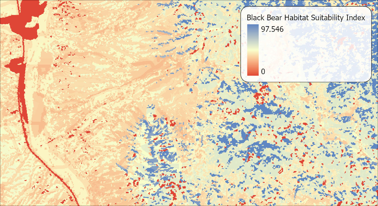
The book's guidance on factors is refreshingly blunt. Prefer categorical metrics with few classes: if a snake is affected by roads out to 200 m and perceives vehicle vibration to 50 m, then three distance-to-road classes (0–50, 50–200, >200 m) capture everything the literature can support — ten classes would just be false precision. Or as the workshop book memorably puts it: our models are crude, and making them more complex is just polishing a turd. Land cover is usually the most important factor and also the most error-ridden (typical classification accuracy 60–80%); lumping closely related classes both matches the literature's resolution and improves effective accuracy. Report your sources and their accuracy — transparency is a hallmark of science.
Factor scores combine by additive (weighted arithmetic mean) or geometric mean algorithms — the geometric mean lets a terrible score on one factor drag the result down toward it, which is often the right behavior for limiting factors. The choice, and its consequences, are covered on the Create Habitat Suitability Model tool's page. Finally, because suitability alone doesn't say whether habitat comes in usable amounts, the workflow maps habitat patches: contiguous areas of good habitat large enough to support breeding (a breeding patch) or a persistent population (a population patch) — the Create Habitat Patches tool's territory, and the raw material for corridor termini.
Corridor modeling
The idea behind the corridor is simple, and worth stating plainly before the mechanics. We want to connect two protected areas — the wildland blocks — so we first find the single best route between them, and then we widen that route into a band of land broad enough to actually conserve. Everything in this section is about how the best route is chosen, and how far out from it the corridor should reach.
“Best” here means least costly for the animal to travel. Picture a bear setting out from one block toward the other. Every pixel it crosses charges a toll: a little energy, a little exposure, some risk of not finding food or cover or of meeting a car. The toll is low in the habitats the species prefers and high in the ones it avoids, and we know which is which from the habitat suitability model we just built — that model is, after all, our best statement of what this species likes and dislikes. Add up the tolls along any route from block to block and you have that route's total cost. The least-cost path is the route with the smallest total — not the shortest line on the map, but the cheapest line for the animal. A path that detours through good habitat can easily beat a straight shot across bad habitat, and that is exactly the behavior we want the model to reward.
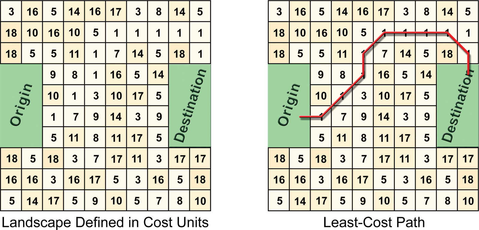
One path a single pixel wide is not a corridor, though. Animals do not walk a line, and a conservation plan cannot protect one. So the last move is to ask, for every pixel in the landscape, “how much more would the cheapest trip cost if it had to pass through you?” Pixels on or near the best route add almost nothing; pixels far out in poor habitat add a great deal. Keeping every pixel whose answer falls below some threshold expands the path outward into a swath — the corridor — and raising the threshold widens it. That is the whole method. From an HSM to a corridor, it takes three steps:
Step 1 — resistance is inverted suitability. Travel cost through a pixel is defined as Resistance = 100 − suitability (on the 0–100 scale). Resistance reflects the ecological cost of crossing a pixel — mortality risk and energetic cost, offset by food, water and cover — not travel speed; animals often move fastest through the worst pixels. (The Invert Raster tool performs exactly this flip; see also the standing guidance on which surfaces are already cost-ready on each tool's page.)
Step 2 — choose termini, and give the model room to run. A terminus is the part of a wildland block where the corridor starts or ends — best chosen as known breeding populations, then modeled population patches, then breeding patches, in that order of preference. Because cost-distance contains plain Euclidean distance, blocks that nearly touch will pull the model toward the narrowest gap regardless of habitat quality; placing termini well inside the blocks (“room to run”) keeps the corridor honest, or at least proves the model's choice wasn't an artifact of geometry.
Step 3 — cost-distance, then slice. Each pixel's cost-distance is the lowest possible cumulative resistance from that pixel to a terminus in each block; unlike raw suitability, cost-distance always forms continuous swaths. The corridor is a slice — the set of pixels below a cost-distance threshold. Slices are nested: as the threshold grows the corridor widens, then sprouts additional strands. Choosing the slice is the hardest judgment in the workflow — wide enough to function (wider than a home-range width for corridor-dwelling species), narrow enough to be conservable. The Least-Cost Corridor tool builds these surfaces and slices without any Spatial Analyst license. Once a slice is drawn, the Bottleneck Analysis tool finds its constrictions — the narrowest places along the corridor. A pinch point is not a wall, but it can be too narrow for a species to move through comfortably, and narrow enough that an animal simply refuses to enter it: too close to the houses, the lights, the noise, the dogs. A slice that looks wide enough on average can be checked at its weakest points before anyone commits to it.
From corridors to a linkage design
The vocabulary matters: a corridor serves one species; the union of all single-species corridors is the preliminary linkage design; and the linkage design is that union after deliberate modification — expanded to serve focal species that never got a corridor model (via their habitat patches, known occurrences, or expert judgment), widened to buffer edge effects and river reaches, and trimmed of redundant strands that add cost without adding function. The final product couples the map with recommendations for crossing structures, barrier mitigation, and land management — lesson 4 made concrete. The Union Corridors and Fill Corridor Holes tools handle the geometric steps, and every least-cost model should end with the sanity check the book insists on: least-cost procedures always produce a best corridor, even when the best is inadequate for the species. That is half the reason the Evaluate Corridors tools exist.
The other half is that the biologically optimum corridor has a way of turning out to be the most valuable land to the developer as well — the same gentle valley bottom, the same river frontage. So the developer, reasonably enough, offers an alternative corridor, and the question becomes whether the alternative is good enough. The evaluation tools let you compare the two on the same terms: patch-to-patch distances, bottleneck widths, the habitat quality inside each. By definition the alternative will score worse, but it may still be good enough to facilitate gene flow between the habitat blocks. That is the best case, and a negotiation worth having. Sometimes, though, the comparison shows that even the biological optimum is unusable for the species, in which case there is no point going further with that linkage, and it is far better to learn that from the numbers than from an empty corridor ten years later. The Corridor Evaluation Tutorial walks through exactly this comparison.
The chapters, as Pro tools
| Workflow stage | Tools in this add-in |
|---|---|
| Habitat suitability | Create Habitat Suitability Model, Combine Habitat Factors, Normalize Existing HSM, Reclassify Features in HSM, Critical Habitat Feature (plus the Create HSM Remap Table window). |
| Patches | Create Habitat Patches — breeding and population patches by geodesic area thresholds. |
| Corridor building | Identify Termini Polygons, Least-Cost Corridor, Fill Corridor Holes, Union Corridors. |
| Evaluation | Patch Analysis, Bottleneck Analysis, Weighted Summary Statistics, Histograms and Statistics, Cross-Tab Statistics. |
| Ancillary | Diversity Indices, Invert Raster, Clip Data to Analysis Area, Cumulative Surface, and the Corridor Analysis Data Report. |
| Climate-change-robust alternative | The Land Facet tools (Clustering, Density, Mahalanobis) model corridors on enduring physical terrain rather than present-day vegetation — see About Land Facets. |
Unlike the original ArcMap extension, every tool here runs at every ArcGIS Pro license level — no Spatial Analyst required anywhere in the chain.
Credits and references
The CorridorDesigner approach and the workshop book are by Paul Beier, Dan Majka and Jeff Jenness; the ArcGIS Pro tools are by Jeff Jenness, Jenness Enterprises (www.jennessent.com). The CorridorDesigner project was funded by a grant from the ERDENE initiative at Northern Arizona University.
- Beier, P., D. Majka, and J. Jenness. 2007, revised 2026. Designing wildlife corridors with ArcGIS: ArcGIS Pro edition. Workshop book, revised by J. Jenness for the Corridor Designer Tools of the Wildlife and Forestry Tools add-in. Available at: CorridorDesigner_WorkshopBook_2026_ArcGISPro.pdf (5 MB)
- Beier, P., D. Majka, and J. Jenness. 2007. Designing wildlife corridors with ArcGIS. Workshop book, Northern Arizona University. Available at: corridordesign.org (archived copy at the Internet Archive)
- Beier, P., D. R. Majka, and W. D. Spencer. 2008. Forks in the road: choices in procedures for designing wildland linkages. Conservation Biology 22:836–851. doi.org/10.1111/j.1523-1739.2008.00942.x
- Horskins, K., P. B. Mather, and J. C. Wilson. 2006. Corridors and connectivity: when use and function do not equate. Landscape Ecology 21:641–655. doi.org/10.1007/s10980-005-5203-6
- Majka, D., J. Jenness, and P. Beier. 2007. CorridorDesigner: ArcGIS tools for designing and evaluating corridors. Available at: corridordesign.org (archived copy at the Internet Archive)
Related tools and pages
- The Corridor Design Tutorial, Corridor Evaluation Tutorial and Land Facet Tutorial — the concepts on this page, run end to end on the tools.
- About Land Facets — the terrain-based, climate-change-robust companion to this approach.
- The tool pages listed in the table above — the sidebar carries the full set.
- About Mahalanobis distances — the statistical engine behind the Land Facet corridor approach.