

Land Facet Mahalanobis
Summary
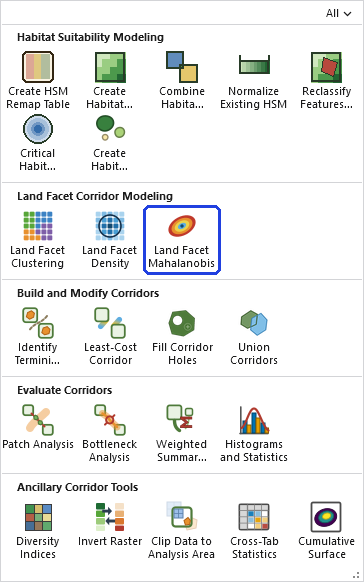
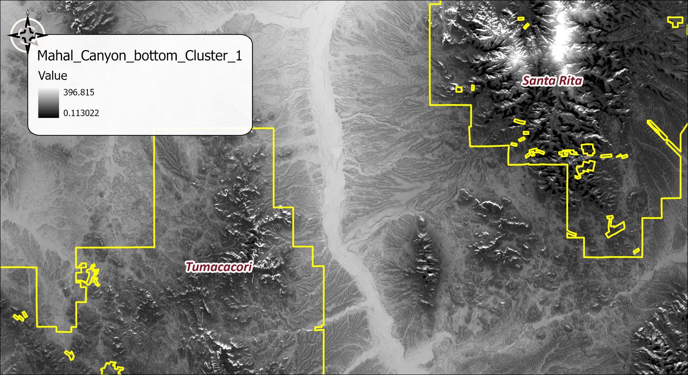
One Mahalanobis distance cost surface per land facet: how far every cell on the landscape departs, in multivariate standard deviations, from the conditions typical of that facet. The third step of a Land Facet corridor analysis, after Land Facet Clustering and Land Facet Density. Low scores mark ground most like the facet — exactly what a least-cost model wants as resistance, so each facet's output raster feeds Least-Cost Corridor directly, with no inversion. No Spatial Analyst needed.
Trained inside the blocks, evaluated everywhere
Each facet's mean vector and covariance matrix come only from the facet's cells inside the Wildland Blocks — places known to support a working natural community, acting as training data — while the surface is evaluated over the whole analysis area, because a corridor has to cross the ground between the blocks and we need to find where block-quality ground occurs out there. For this tool, “Best” means most like what exists in the protected Wildland Blocks.
Why Mahalanobis rather than plain distance? The variables live in different units and are usually correlated — elevation in meters, steepness in degrees, density as a proportion — and a plain Euclidean distance would let whichever variable has the biggest numbers dominate. Mahalanobis distance normalizes by the variances and covariances, so every variable speaks with a fair voice (the full story is on the About Mahalanobis page). When a density raster is supplied, density joins the analysis with a characteristic value of 100% rather than its mean, as the Land Facet method requires — the ideal cell is thoroughly surrounded by its own facet.
The tool validates its inputs' provenance records — a density raster from a different clustering run is refused rather than warned about, because a wrong band produces plausible-looking nonsense — and each facet's optional mean and covariance tables can be saved for inspection.
A tour of the dialog
The example is Step 3 of the Land Facet Tutorial: eighteen facets, three variables and the density raster from the previous step, with the two wildland blocks as the training polygons.
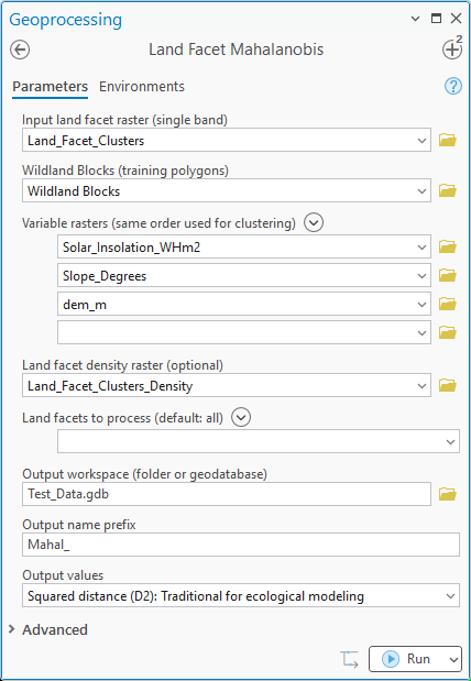
The tool holds all of its raster data in memory at once, so the memory it needs grows with the number of cells. On most rasters that is no concern. On a very large one the tool may need more memory than your computer has free, and then one of two things happens: Windows starts using the disk as overflow memory and the tool slows to a crawl, or the tool stops with an out-of-memory error. There is no fixed limit; it depends on how much memory your computer has free. If your rasters are too large, clip them to the area you need first.
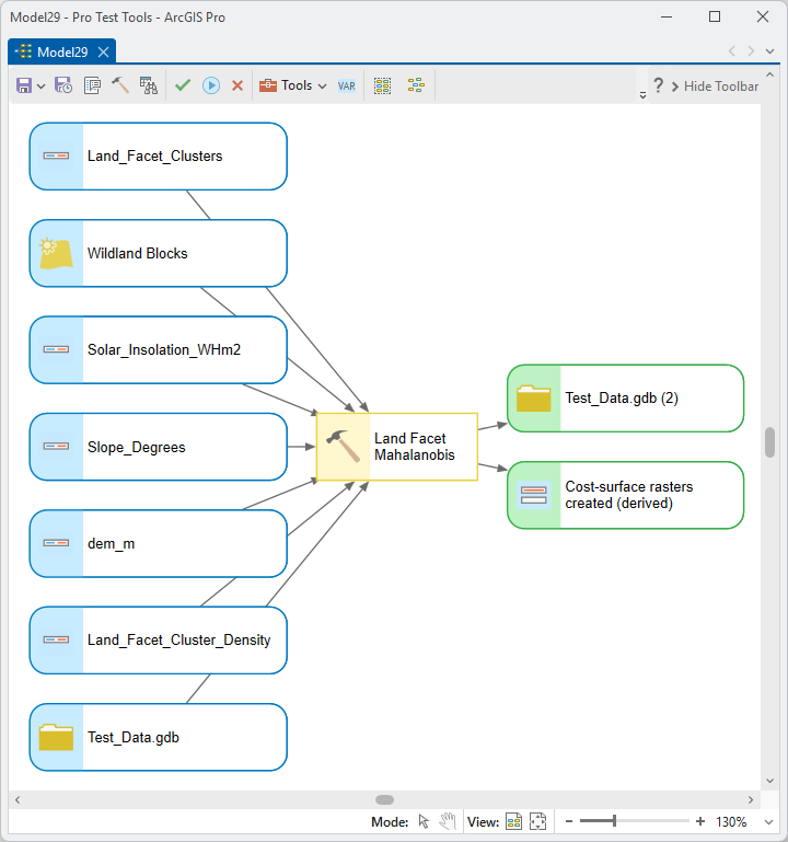
ModelBuilder
Parameters
| Label | Explanation | Data type |
|---|---|---|
| Input land facet rasterRequired · in_raster | The clustered facet raster. | Raster Layer |
| Wildland BlocksRequired · blocks | The training polygons. | Feature Layer |
| Variable rastersRequired · variables | The continuous variables, in the same order used for clustering. | Multiple Value |
| Land facet density rasterOptional · density_raster | Joins the analysis with its ideal pinned at 100%; provenance-validated. | Raster Layer |
| Land facets to processOptional · facets | Default: all. | Multiple Value |
| Output workspace / prefixRequired · out_workspace, out_prefix | One single-band cost raster per facet, named from the facet (default prefix Mahal_). | Workspace / String |
| Output valuesRequired · out_type | D² (default), D, or chi-square p-value. | String |
| Covariance inversionOptional · inversion | Standard inverse or SVD pseudo-inverse. | String |
| Save statistics tablesOptional · save_tables | Each facet's mean vector and covariance table, for inspection. | Boolean |
Python
import arcpy
arcpy.ImportToolbox(r"C:\path\to\JennessEnterprisesTools.pyt")  # your install path
arcpy.jenness.LandFacetMahalanobis(
    in_raster=r"D:\lf.gdb\Land_Facets",
    blocks="Wildland_Blocks",
    variables=r"D:\lf.gdb\elev;D:\lf.gdb\slope;D:\lf.gdb\insolation",
    density_raster=r"D:\lf.gdb\Facet_Density",
    out_workspace=r"D:\lf.gdb",
    out_type="Squared distance (D2)")
Recommended citation
Credits and references
By Jeff Jenness, Jenness Enterprises (www.jennessent.com), from the Land Facet Corridor Designer by Jenness, Brost and Beier.
- Beier, P., D. Majka, and J. Jenness. 2007, revised 2026. Designing wildlife corridors with ArcGIS: ArcGIS Pro edition. Workshop book, revised by J. Jenness for the Corridor Designer Tools of the Wildlife and Forestry Tools add-in. Available at: CorridorDesigner_WorkshopBook_2026_ArcGISPro.pdf (5 MB)
- Brost, B. M., and P. Beier. 2012. Use of land facets to design linkages for climate change. Ecological Applications 22:87–103. doi.org/10.1890/11-0213.1
- Jenness, J., B. Brost, and P. Beier. 2013. Land Facet Corridor Designer. Available at: corridordesign.org (archived copy at the Internet Archive)
- Mahalanobis, P. C. 1936. On the generalised distance in statistics. Proceedings of the National Institute of Sciences of India 2(1):49–55. Reprinted 2018 in Sankhyā A 80(Suppl 1):S1–S7. doi.org/10.1007/s13171-019-00164-5
Licensing information
Works at every ArcGIS Pro license level (Basic, Standard, Advanced). No extension licenses are required.
Related tools and pages
- About Land Facet Corridors and the Land Facet Tutorial — the tool in context.
- About Mahalanobis distances — the statistics from first principles.
- Least-Cost Corridor — consumes these cost surfaces directly.