

Land Facet Clustering
Summary
A land facet is a unit of landscape defined by enduring physical traits, chiefly topography and soils: a high-elevation, north-facing, steep slope on rocky soil, say, or a low flat with deep soil. Facets are the stage on which vegetation grows, and because they do not move when the climate does, a linkage that keeps a continuous strand of each facet should keep a strand of whatever vegetation the future puts on it (Beier and Brost 2010). This tool is where the facets are defined.
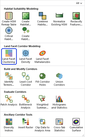
Defines the land facets: an interactive window that runs the fuzzy c-means clustering workflow of the Land Facet Corridor Designer entirely inside ArcGIS Pro — the step that originally required exporting tables to R, running a package of R functions, and importing the results back. Give it a first-pass classification raster (topographic position, soil type, or a single class covering everything), your continuous variables (elevation, slope, insolation, soil properties), and the wildland blocks; it screens multivariate outliers, clusters each class across candidate cluster counts, screens poorly classified cells by their confusion index, and writes one combined raster of uniquely numbered land facets with interpretable names. The numerics are validated against the original published R implementation.
Handling everything internally does not close the door on R. The window's Export tables for R... button writes the same tables the original Export-for-R tool did, one CSV per class in the same schema, from the same data it has just read. So if you would rather run the clustering in R, or want to check this window's results against the original functions, you can take the tables there exactly as before.
The workflow inside the window
Following Beier and Brost's procedure: facets are defined from the cells inside the wildland blocks (they should represent what the linkage connects); within each first-pass class, cells with rare combinations of the continuous variables are removed as outliers (they would stretch clusters across empty attribute space); fuzzy c-means then finds the natural groupings for each candidate number of clusters, and the goodness-of-fit metrics offer evidence on how many clusters are most statistically defensible for each class, the cluster count that best matches the landscape's real multivariate “lumpiness.” The metrics do not always agree with one another, and you can always set the number of clusters yourself. Cells that assign with nearly equal probability to two facets are dropped by the confusion screen: they are excluded from the rest of the analysis and end up as NoData cells in the land facet raster, along with the outliers, leaving distinctive facets. Batch mode processes all first-pass classes into one combined raster with unique facet IDs, symbolized by class, with a class-name field ready for legends.
The output raster carries the analysis record that the rest of the chain validates — Land Facet Density, Land Facet Mahalanobis, and the corridor tools all check their inputs descend from the same clustering run.
A tour of the window
The example is Step 2 of the Land Facet Tutorial. Here we have already used the Slope Position Classification tool to classify the landscape into canyon bottoms, flat-gentle slopes, steep slopes and ridgetops from the elevation and slope across the landscape. Now we generate land facet clusters within each of these four classes, clustering on elevation, slope and annual solar insolation, using only the cells inside the two wildland blocks to define them. The window is a four-page wizard, and pages 2 and 3 are worked once for each class before page 4 can write the raster.
Page 1: Setup
Page 2: Outliers
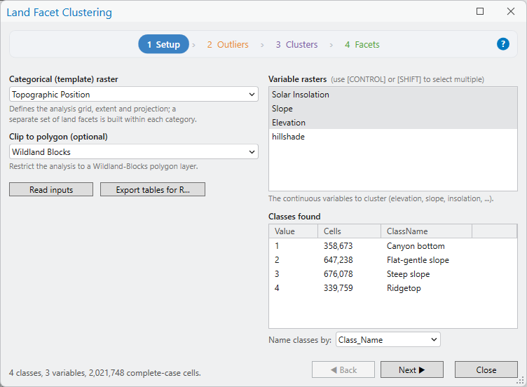
An outlier here is a cell with a rare combination of the variables: not an extreme value of any one of them, but a point that sits alone in the multivariate space, such as an unusually high, flat and sunny canyon bottom. Left in, such cells stretch the clusters across empty attribute space and pull the cluster centers toward ground that barely exists. The page draws a sample of the class (4,000 cells here), estimates the density of the sample around each point using all the variables at once, and flags the least-dense fraction as outliers. The Outlier fraction is yours to set: drag the slider or type a percentage into the box (10% is the default and the original work's choice). The outliers are set aside from the clustering on the next page, so the clusters describe the common ground, and they are left NoData in the facet raster, since a cell that belongs to no facet should not be forced into one.
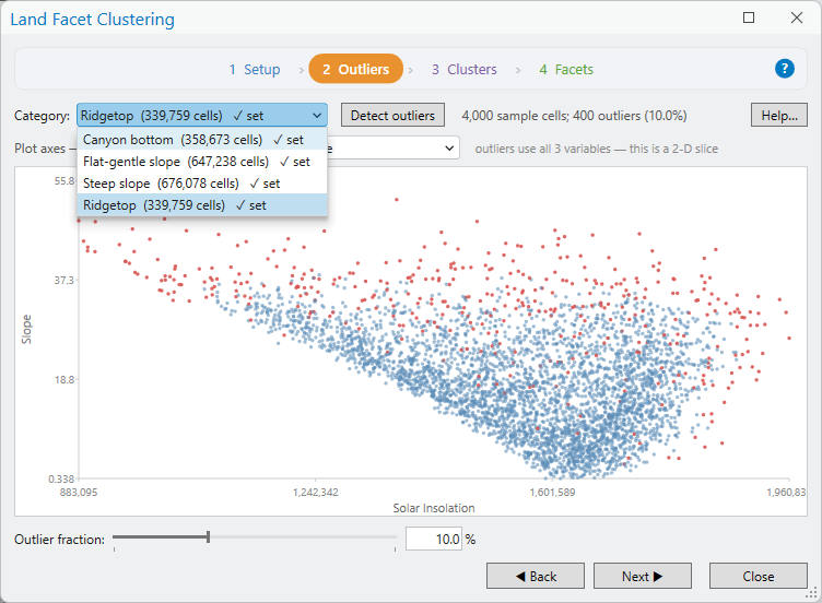
The plot can only show two variables at a time, but the outliers were found using all of them. Change the Plot axes to look at the same sample from another direction.
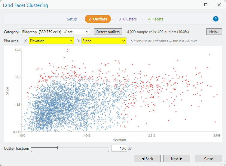
Before moving on, run Detect outliers for every category you intend to cluster. Once it has run for a category, the word set with a check mark is added after that category's name in the list, so you can see at a glance which classes are done and which are still waiting. Page 3 works the same way, with its own set marks for the clustering.
Page 3: Clusters
Again one class at a time: choose the category and click Run clustering. The window runs fuzzy c-means on the non-outlier sample for every candidate number of clusters from 2 to 7, with the fuzziness and the number of random restarts shown in the boxes, and plots eight cluster-validity indices against the number of clusters. A consensus vote of the six clearest indices picks the suggested count, and the dashed line marks the count currently chosen on every chart.
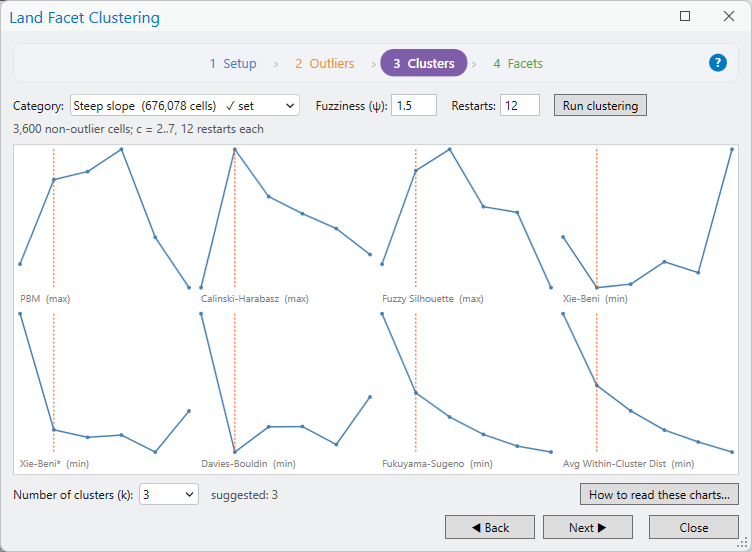
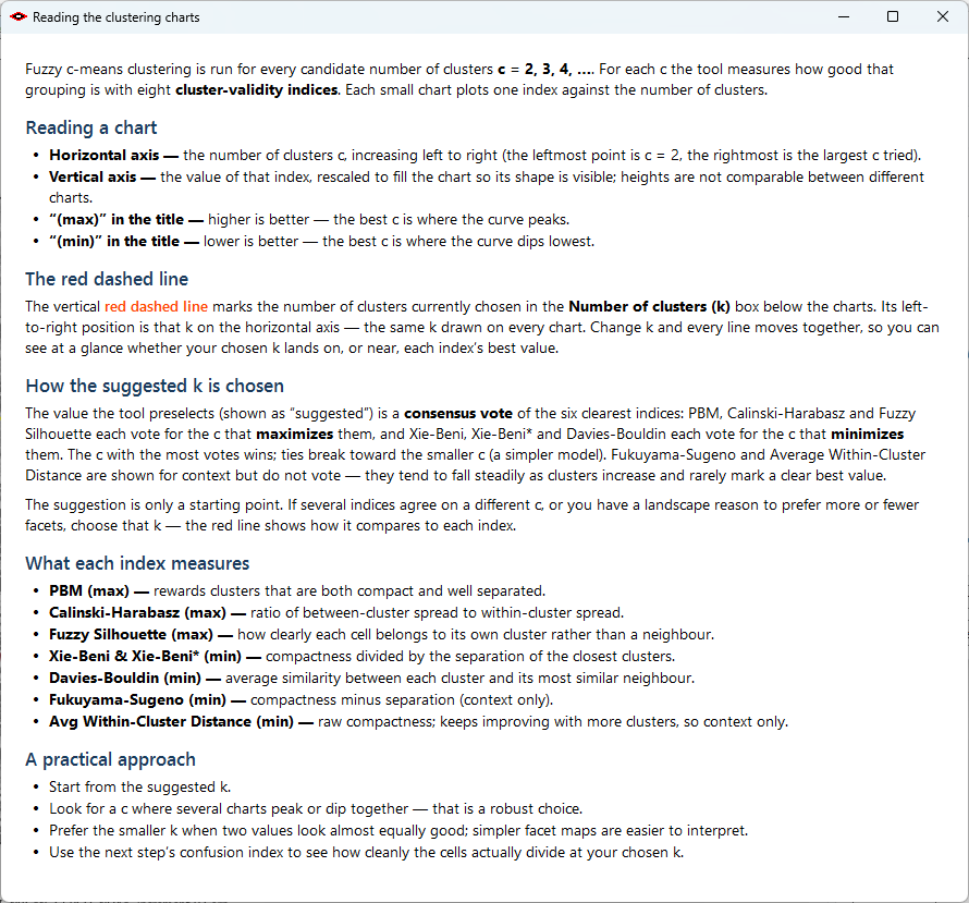
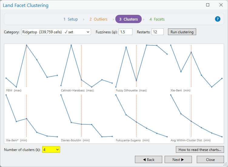
The charts steer the suggestion; they do not make the decision. The Number of clusters box can be set to any count, and the dashed line moves to show how that count sits against every index. In the tutorial, ridgetops were suggested six clusters and were given four.
Page 4: Facets
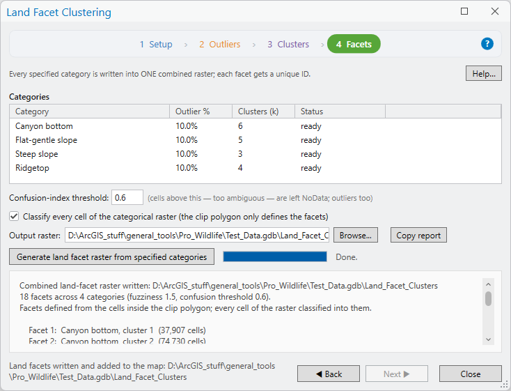
The report, copied out in full from the tutorial run. The analysis id at the end is the record the downstream tools read, so the facet list and the variable order never have to be typed again.
Combined land-facet raster written: D:\ArcGIS_stuff\general_tools\Pro_Wildlife\Test_Data.gdb\Land_Facet_Clusters
18 facets across 4 categories (fuzziness 1.5, confusion threshold 0.6).
Facets defined from the cells inside the clip polygon; every cell of the raster classified into them.

    Facet 1:  Canyon bottom, cluster 1  (37,907 cells)
    Facet 2:  Canyon bottom, cluster 2  (74,730 cells)
    Facet 3:  Canyon bottom, cluster 3  (49,176 cells)
    Facet 4:  Canyon bottom, cluster 4  (217,386 cells)
    Facet 5:  Canyon bottom, cluster 5  (90,142 cells)
    Facet 6:  Canyon bottom, cluster 6  (79,093 cells)
    Facet 7:  Flat-gentle slope, cluster 1  (353,443 cells)
    Facet 8:  Flat-gentle slope, cluster 2  (16,578 cells)
    Facet 9:  Flat-gentle slope, cluster 3  (1,122,451 cells)
    Facet 10:  Flat-gentle slope, cluster 4  (895,797 cells)
    Facet 11:  Flat-gentle slope, cluster 5  (348,083 cells)
    Facet 12:  Steep slope, cluster 1  (237,017 cells)
    Facet 13:  Steep slope, cluster 2  (944,138 cells)
    Facet 14:  Steep slope, cluster 3  (246,193 cells)
    Facet 15:  Ridgetop, cluster 1  (105,499 cells)
    Facet 16:  Ridgetop, cluster 2  (224,477 cells)
    Facet 17:  Ridgetop, cluster 3  (130,372 cells)
    Facet 18:  Ridgetop, cluster 4  (69,674 cells)

Analysis metadata recorded (id 52be593e-7e63-45d2-883c-90025e5fe45a). The Land Facet Density and Mahalanobis tools will read the facet list and variable order from this raster.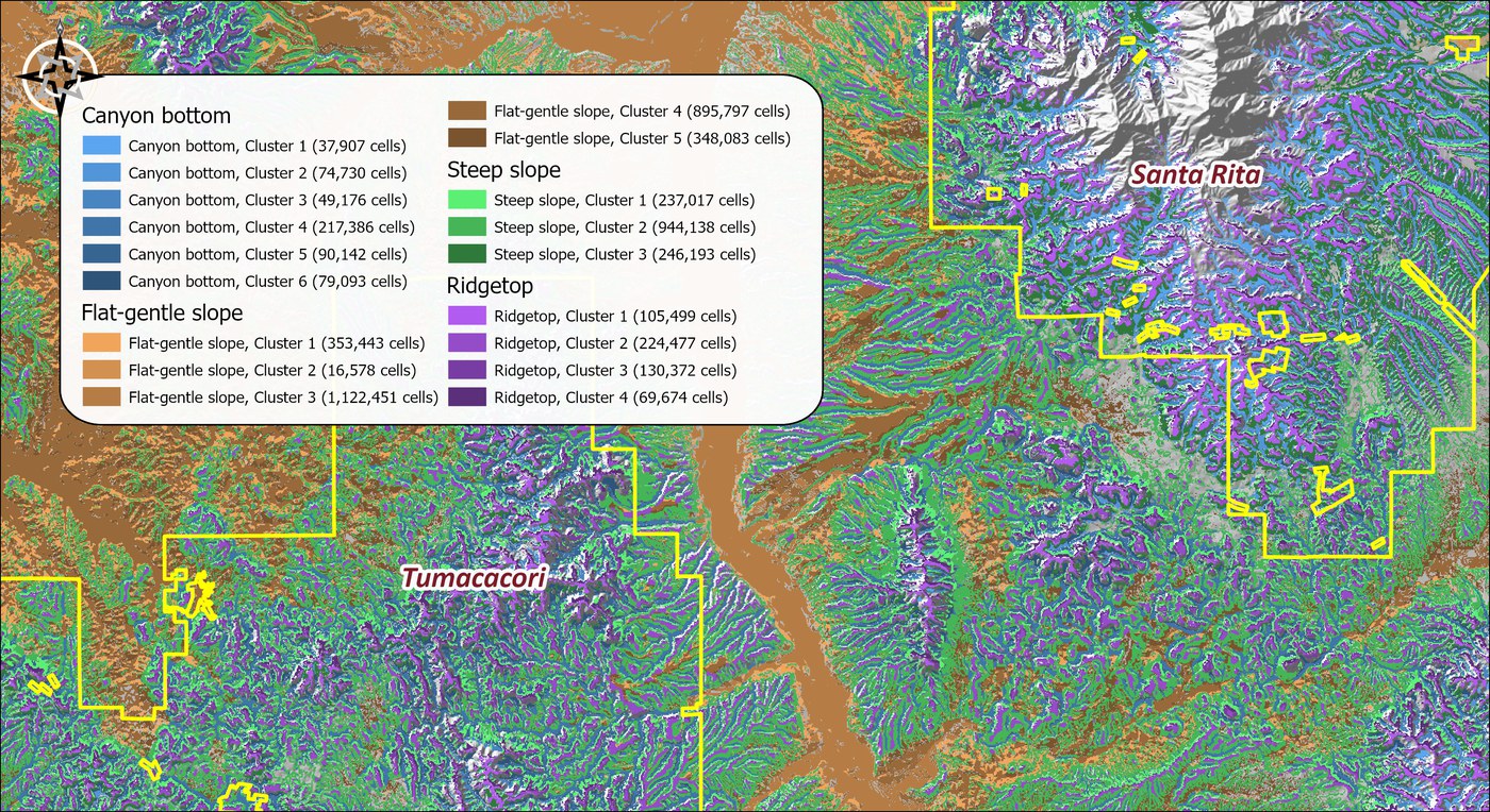
Recommended citation
Credits and references
By Jeff Jenness, Jenness Enterprises (www.jennessent.com), from the Land Facet Corridor Designer by Jenness, Brost and Beier; fuzzy c-means after Bezdek.
- Beier, P., and B. Brost. 2010. Use of land facets to plan for climate change: conserving the arenas, not the actors. Conservation Biology 24:701–710. doi.org/10.1111/j.1523-1739.2009.01422.x
- Bezdek, J. C. 1981. Pattern recognition with fuzzy objective function algorithms. Plenum Press, New York. doi.org/10.1007/978-1-4757-0450-1
- Brost, B. M., and P. Beier. 2012. Use of land facets to design linkages for climate change. Ecological Applications 22:87–103. doi.org/10.1890/11-0213.1
Licensing information
Works at every ArcGIS Pro license level (Basic, Standard, Advanced). No extension licenses are required — and no R installation.
Related tools and pages
- About Land Facet Corridors — why facets, and the five Major Steps.
- Land Facet Tutorial — the window in the full workflow.
- Land Facet Density — the next step in the chain.
- Diversity Indices — measures the diversity of the facet raster this window writes, for the interspersion corridor.