About Mahalanobis Distances

Home Range · background and theory · by Jeff Jenness

This page covers the ideas shared by the four Mahalanobis tools — Mahalanobis Distance Raster, Mahalanobis Distance at Points, Calculate Statistical Matrices, and Mahalanobis Chi-Square Transform — so each tool's page can concentrate on its own controls. The discussion is adapted from the manual Jeff wrote for his original, award-winning ArcView Mahalanobis Distances extension.

Measuring similarity to ideal conditions

Mahalanobis distances provide a powerful method of measuring how similar some set of conditions is to an ideal set of conditions, and can be very useful for identifying which regions in a landscape are most similar to some “ideal” landscape.

For example, in the field of wildlife biology we might define an “ideal” landscape as that which best fits the niche of some wildlife species. Through observation, we may find that a wildlife species typically occurs within a particular elevation range, on slopes of a particular steepness, and perhaps within a certain vegetation density. Using Mahalanobis distances, we can quantitatively describe the entire landscape in terms of how similar it is to the ideal elevation, slope and vegetation density of that animal.

Moreover, Mahalanobis distances are based on both the mean and variance of the predictor variables, plus the covariance matrix of all the variables, and therefore take advantage of the covariance among variables. Suppose our hypothetical species likes steep slopes at low elevations and shallow slopes at high elevations: that implies a certain covariance relationship between slope and elevation, and the Mahalanobis distance for a sample will be based on that relationship — so we won't inadvertently select steep slopes at high elevations or shallow slopes at low elevations. The region of constant Mahalanobis distance around the mean forms an ellipse in 2-D space (when only 2 variables are measured), or an ellipsoid or hyperellipsoid when more variables are used.

The formula

Mahalanobis distances are calculated as:

D^{2} = {(x - m)}^{T} C^{- 1} (x - m)

where D² is the squared Mahalanobis distance; x is the vector of data values; m is the vector of mean values of the independent variables; C⁻¹ is the inverse covariance matrix of the independent variables; and T indicates that the vector should be transposed. The tools can report the squared distance D² (the quantity traditionally mapped in ecological models), its square root D (the literal distance, analogous to Euclidean distance), or a chi-square p-value derived from D² (below).

A worked example

Suppose we took a single observation from a bivariate population with Variable X and Variable Y, where X has mean = 500, SD = 79.32 and Y has mean = 500, SD = 79.25, with this variance/covariance matrix:

Variance/Covariance Matrix
	X	Y
X	6291.55737	3754.32851
Y	3754.32851	6280.77066

If our single observation has X = 410 and Y = 400, then:

(x - m) = (\begin{matrix} 410 - 500 \\ 400 - 500 \end{matrix}) = (\begin{matrix} - 90 \\ - 100 \end{matrix})

C^{- 1} = {(\begin{matrix} 6291.55737 & 3754.32851 \\ 3754.32851 & 6280.77066 \end{matrix})}^{- 1} = (\begin{matrix} 0.000247 & - 0.000148 \\ - 0.000148 & 0.000248 \end{matrix})

D^{2} = (\begin{matrix} - 90 & - 100 \end{matrix}) (\begin{matrix} 0.000247 & - 0.000148 \\ - 0.000148 & 0.000248 \end{matrix}) (\begin{matrix} - 90 \\ - 100 \end{matrix}) = 1.818

Therefore, our single observation lies a squared distance of 1.818 standardized units from the mean (the mean being at X = 500, Y = 500). (Carrying full precision through the matrix inverse gives 1.818; the 2005 manual's 1.825 came from multiplying through the rounded inverse shown there.)

If we took many such observations, graphed them, and colored them according to their Mahalanobis values, we can watch the elliptical Mahalanobis regions come out. The cloud below is randomly generated from the bivariate population described above — the points are normally distributed along two major axes of variance, with the standard deviation along the primary axis set to twice that of the secondary axis:

A scatter cloud of twenty thousand normally distributed random points forming a tilted elliptical cluster centered at 500, 500 — 20,000 random observations from the bivariate population.

The same cloud with its two diagonal axes of variance drawn through the centroid at 500, 500, the primary axis with standard deviation 100 and the secondary with 50 — The same cloud with its centroid and its two axes of variance (primary SD = 100, secondary SD = 50).

The cloud shaded by Mahalanobis distance value, green at the center grading through yellow and red to dark red at the fringes in clear elliptical bands — Each point shaded by its Mahalanobis distance: clear elliptical patterns emerge.

The cloud overlaid with concentric ellipses drawn at constant Mahalanobis distances from one half through ten — Ellipses drawn at constant squared Mahalanobis distances (D²).

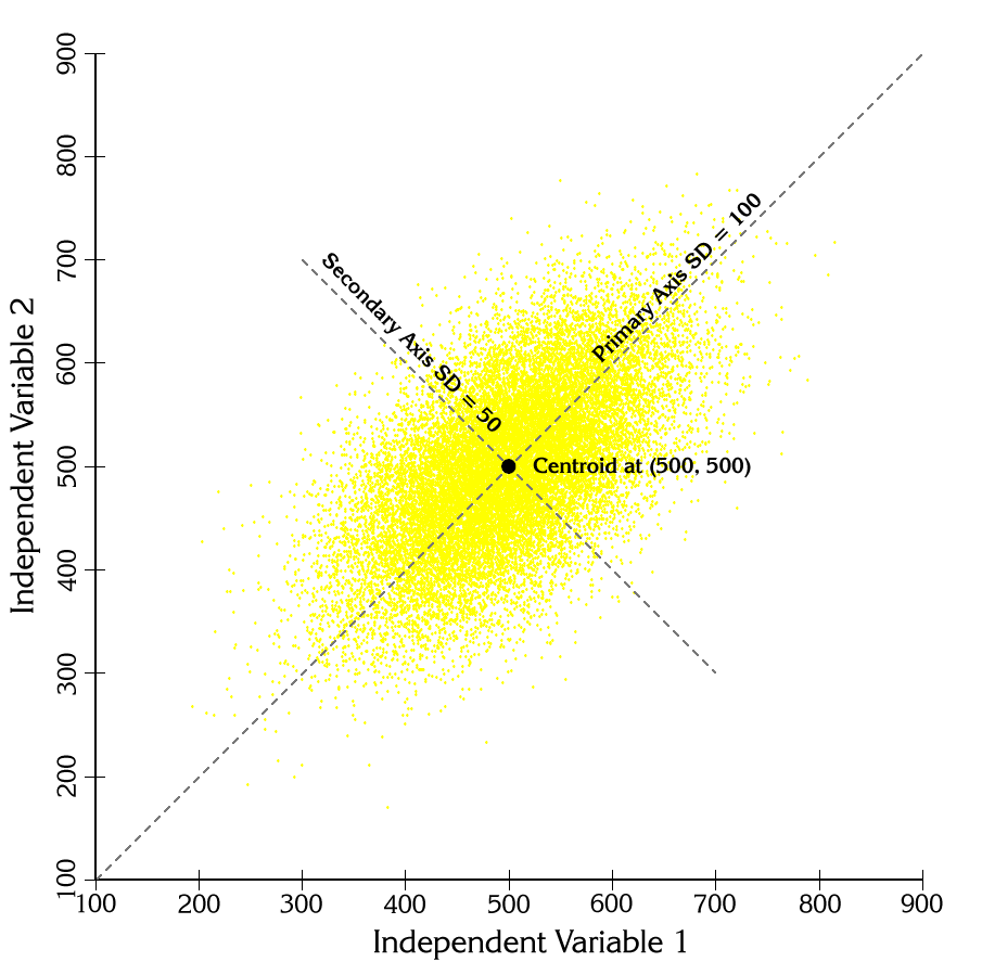
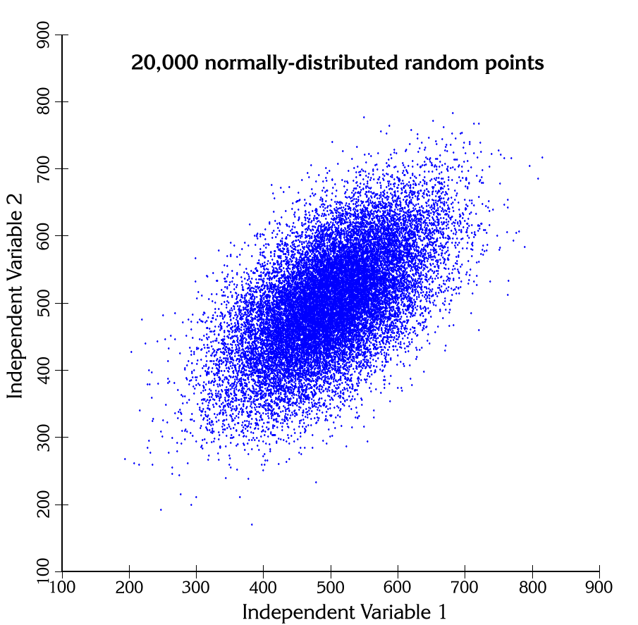
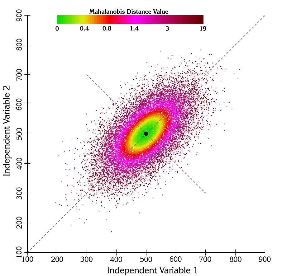
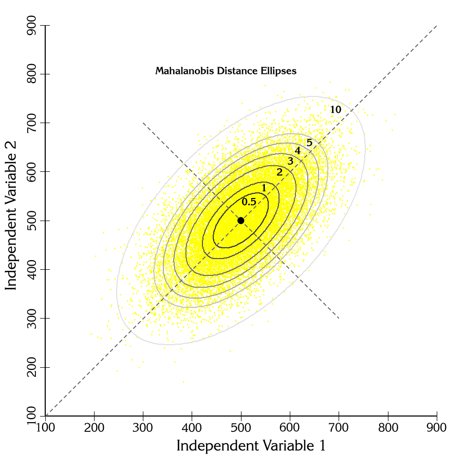
One interesting feature to note from this figure: the ellipse labeled 1 crosses each major axis of variance at exactly 1 standard deviation from the mean. The value 1 is special that way — since 1² = 1, the distinction between the distance D and the squared distance D² vanishes there, and the statement is true whichever quantity you map. Farther out, the crossing point follows the square root of the labeled D² value: the ellipse labeled 4 sits 2 standard deviations out along each axis, and the ellipse labeled 10 about 3.2. (Measure the figure and you'll see it — the 10 ellipse reaches roughly 316 units along the primary axis, whose standard deviation is 100.)

Chi-square p-values

Mahalanobis distances are occasionally converted to chi-square p-values for analysis (see Clark et al. 1993). When the predictor variables are normally distributed, the squared distances follow a chi-square distribution — and even when they are not (Farber and Kadmon 2003 warn that wildlife habitat variables often fail the normality assumption), the conversion still serves to recode the distances onto a fixed 0 to 1 scale. Mahalanobis distances themselves have no upper limit, so this rescaling can be convenient.

The p-value reflects the probability of seeing a Mahalanobis value as large or larger than the actual value, assuming the vector of predictor values was sampled from a population with the ideal mean. P-values close to 0 reflect high Mahalanobis distances — very dissimilar to the ideal combination of predictor variables; p-values close to 1 reflect low distances — very similar to the ideal. The closer to 1, the more similar.

Which degrees of freedom? The statistically standard result is that D² follows a chi-square distribution with degrees of freedom equal to the number of variables (Mardia, Kent and Bibby 1979; Seber 1984) — two variables, two degrees of freedom. Some influential ecological sources instead used the number of variables minus one (Clark et al. 1993; Farber and Kadmon 2003), and Jeff's original ArcView extension followed that convention. These tools use the standard value — but because the chi-square transform is monotonic in D², the choice only rescales the p-values and never changes the ranking of cells or points, and the Chi-Square Transform tool lets you set the degrees of freedom yourself if you wish to reproduce those sources.

Applications to landscape analysis

The Mahalanobis equation doesn't care whether x is a vector of numbers or a vector of whole rasters: supply a raster per variable and the arithmetic produces a raster of Mahalanobis values, describing every cell's similarity to the reference conditions. That is exactly what the Mahalanobis Distance Raster tool does. (The 2005 manual noted an eight-raster limit in ArcView Spatial Analyst; the Pro tools compute the quadratic form directly in blocks, with no variable limit — and no Spatial Analyst license at all.)

Suppose we have a set of animal locations plus rasters of elevation and slope, and we want to identify regions on the landscape similar to the conditions at the animal locations — potential habitat, in other words:

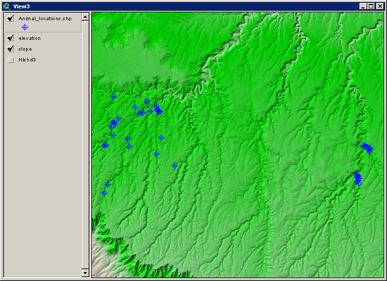
A hillshaded terrain map with a cluster of blue animal location points along a drainage — Animal locations over the landscape. For the curious, this map window dates back to ArcView 3.x, way back in the misty dawn of GIS — a dark and distant age, only dimly remembered now.

We use the points to generate the mean vector and covariance matrix of elevation and slope at the locations, then evaluate the whole landscape against those statistics:

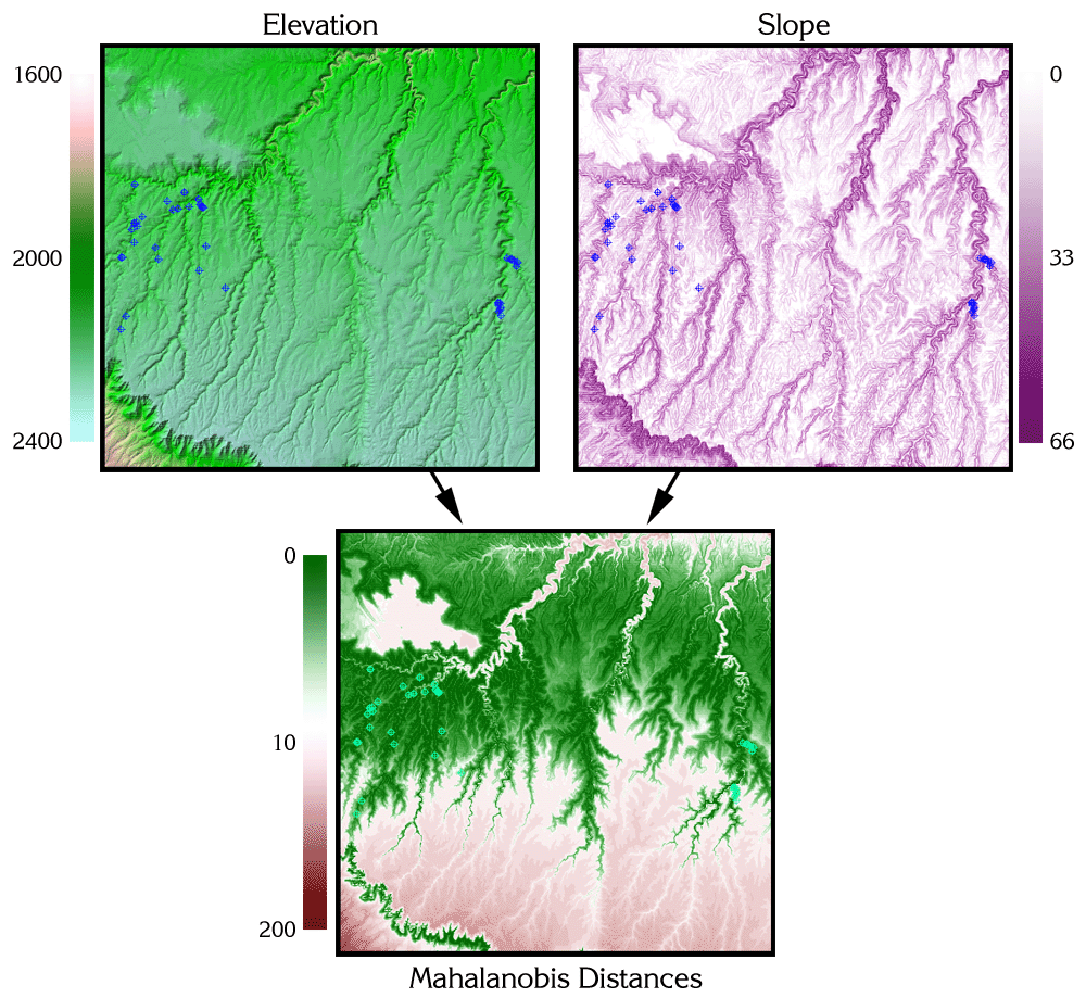
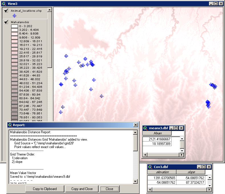
An elevation raster and a slope raster combining into a Mahalanobis distance raster whose lowest values trace the terrain most similar to the sample conditions — Elevation and slope in, Mahalanobis distances out: low values mark ground most similar to the conditions at the sample points.

The resulting Mahalanobis surface with the sample points overlaid, low-distance similar terrain shown bright — The Mahalanobis surface: a similarity map of the whole landscape.

Using categorical data

Categorical data do not lend themselves directly to Mahalanobis analysis: the ideal vector is composed of the means of the variables involved, and it is difficult to find the mean of a set of categories. But there are aspects of categorical datasets that work well. Clark et al. (1993) derived a numeric diversity raster from their categorical map, where each cell holds the number of distinct categories within a neighborhood — in ArcGIS Pro, Focal Statistics with the Variety statistic, or our own Diversity Indices tool. Another option is a proportion-of-neighborhood raster per category of interest: query the categorical raster for one category (1/0), take a focal Sum over your neighborhood, and divide by the neighborhood's cell count. Either derivative is a reasonable continuous variable for the Mahalanobis analysis.

The four tools, and how they fit together

Mahalanobis Distance Raster is the landscape workhorse: variables in (rasters, multiband rasters, or polygon fields), reference statistics from sample points, a categorical raster, or saved tables — and a surface of D², D, or p-values out. Mahalanobis Distance at Points evaluates the same quantity at point features instead of every cell — each point's distance from the reference conditions, written to fields. Calculate Statistical Matrices is the producer: it computes the mean vector, covariance, inverse covariance, and correlation tables once, for reuse by the other tools (and for inspecting collinearity). Mahalanobis Chi-Square Transform rescales a D² raster to the 0 to 1 p-value surface.

One warning shared by the whole suite: variable order matters. The variables become the columns of the mean vector and covariance matrix in the order listed, and reusing saved statistics with the variables in a different order silently produces incorrect distances — we don't want our elevation values evaluated against our slope mean and variance! The tools in this add-in help you avoid this problem by writing the variable order into the saved tables' metadata, so the other tools in the add-in know automatically what order to analyze the variables in — and can warn you if the variables you supply don't match. If you intend to use statistical tables you generated from other sources, though, that safety net isn't there: you'll just need to take care to put the variables in the correct order yourself.

References

Clark, J. D., J. E. Dunn, and K. G. Smith. 1993. A multivariate model of female black bear habitat use for a geographic information system. Journal of Wildlife Management 57:519–526. doi.org/10.2307/3809276
Farber, O., and R. Kadmon. 2003. Assessment of alternative approaches for bioclimatic modeling with special emphasis on the Mahalanobis distance. Ecological Modelling 160:115–130. doi.org/10.1016/S0304-3800(02)00327-7
Knick, S. T., and D. L. Dyer. 1997. Distribution of black-tailed jackrabbit habitat determined by GIS in southwestern Idaho. Journal of Wildlife Management 61:75–85. doi.org/10.2307/3802416
Mahalanobis, P. C. 1930. On tests and measures of group divergence. Journal and Proceedings of the Asiatic Society of Bengal 26:541–588. (The paper the 1936 classic itself points back to for the origin of D².)
Mahalanobis, P. C. 1936. On the generalised distance in statistics. Proceedings of the National Institute of Sciences of India 2(1):49–55. Reprinted 2018 in Sankhyā A 80(Suppl 1):S1–S7. doi.org/10.1007/s13171-019-00164-5
Mardia, K. V., J. T. Kent, and J. M. Bibby. 1979. Multivariate analysis. Academic Press, London.
Seber, G. A. F. 1984. Multivariate observations. John Wiley and Sons, New York.

For the underlying matrix algebra and computational algorithms, Jeff also recommends:

Conover, W. J. 1980. Practical nonparametric statistics, 2nd ed. John Wiley and Sons. 493 p.
Draper, N. R., and H. Smith. 1998. Applied regression analysis, 3rd ed. Wiley Series in Probability and Statistics. 706 p.
Golub, G. H., and C. F. Van Loan. 1996. Matrix computations, 3rd ed. Johns Hopkins University Press. 694 p.
Meyer, C. D. 2000. Matrix analysis and applied linear algebra. Society for Industrial and Applied Mathematics, Philadelphia. 718 p.
Neter, J., W. Wasserman, and M. H. Kutner. 1990. Applied linear statistical models, 3rd ed. Richard D. Irwin, Homewood, Illinois. 1181 p.
Press, W. H., S. A. Teukolsky, W. T. Vetterling, and B. P. Flannery. 2002. Numerical recipes in C: the art of scientific computing, 2nd ed. Cambridge University Press, Cambridge. 994 p.

Mahalanobis Distance Raster, Mahalanobis Distance at Points, Calculate Statistical Matrices, and Mahalanobis Chi-Square Transform — the four tools this page underpins.
The Land Facet Mahalanobis tool (Corridor Designer Tools) applies the same distances per land facet to build corridor cost surfaces.