

Corridor Design Tutorial
This tutorial walks the standard CorridorDesigner workflow end to end — from raw statewide data to a modeled corridor for a single focal species — using the ArcGIS Pro tools in this add-in. It is adapted from Chapter 6 of the 2007 workshop book Designing Wildlife Corridors with ArcGIS; the concepts behind every step are on the About Corridor Design page. The original tutorial required an ArcInfo-level license with Spatial Analyst; this chain runs at every ArcGIS Pro license level. The workshop book itself has been revised to match: the 2026 ArcGIS Pro edition (PDF, 5 MB) keeps the 2007 text of Chapters 1–5 and the appendices unchanged and replaces Chapter 6 with this tutorial, condensed for print.
Corridor_Tutorial_Data folder you will find:
Corridor_Tutorial_Data.gdb— the input datasets for the analysis area: the DEM (dem_m), the Arizona GAP land cover (aml_landcover), roads, the interstate, streams, land ownership, and the wildland blocks. Also a county parcel map (Parcels_in_Region, 26,199 parcels) for the Corridor Evaluation Tutorial; the owner names have been replaced with anonymous labels such as Individual Owner #12 or Corporate Owner #3, with anOwner_Typefield to sort them, and the addresses removed — public agencies keep their real names.speciesData\blackbear\— the black bear expert's scores as template files for the Create HSM Remap Table window, one per habitat factor (blackbear_elev_m.txt,blackbear_lndcvr.txt,blackbear_topo.txt,blackbear_dstroad.txt), plus the factor weights (blackbear_weights.txt), the patch parameters (blackbear_patches.txt) and the original rating form the scores came from.- The rest of
speciesData\— the same set of files for eleven other species we modeled when these tools were first developed, one folder each: antelope jackrabbit, Arizona gray squirrel, badger, coati, Coues white-tailed deer, jaguar, javelina, mountain lion, mule deer, porcupine and tiger rattlesnake. Once you have run the tutorial for black bear, any of them can be run the same way, and together they show how differently a dozen species read the same four factors. Ancillary_Files\— what the 46 land cover codes mean: the class list as a spreadsheet and the Arizona GAP vegetation description appendix. You will want these open when you score land cover.Workshop_Slides\— PDF copies of the six slide decks from the CorridorDesigner workshops (the big picture, habitat modeling, patch modeling, corridor modeling, sensitivity analysis and evaluating corridors). The workshop book's Chapter 5 exercises refer to slides in the first two.- Arizona CorridorDesigner Toolbox Documentation (PDF, 1 MB, also included in the zip) — the 2007 species accounts by Majka, Jenness and Beier. For each of the 28 Arizona focal species, mammals through amphibians and reptiles, it records how the habitat criteria were defined: which factors were used, how each factor's classes were scored, the factor weights, and the patch sizes, with the reasoning and sources behind them. This is where the numbers in the template files come from, and the model to follow when you document a species of your own.
Step 1: Define the analysis area and wildland blocks
Set up a project folder with a basemap home for input layers and an output home for everything the models produce — a corridor analysis for even one species spawns dozens of datasets, and a naming convention (species name as a prefix, thresholds in file names) pays for itself immediately.
Create a polygon feature class for the analysis area and digitize a generous rectangle around both wildland blocks — with enough matrix on all sides that a looping corridor has room to exist. Then create the two wildland block polygons, typically by selecting and exporting the appropriate ownership polygons (the Forest Service blocks here). The blocks anchor the whole analysis: the corridor will connect habitat within them.
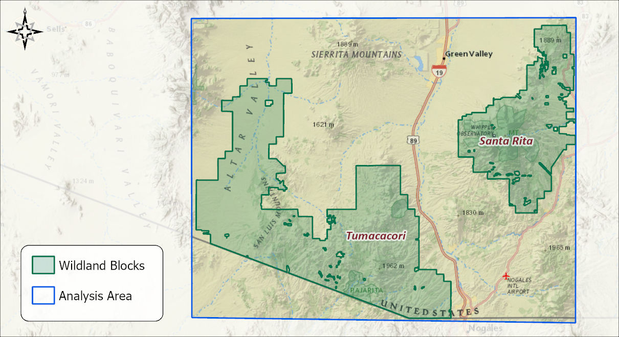
Step 2: Clip the analysis layers
Gather every layer the models will touch — land cover, elevation, roads, streams, ownership — and clip them all to the analysis area in one pass with Clip Data to Analysis Area. Clipping shrinks processing time, keeps intermediate rasters small, and produces a self-contained project you can hand to partners. From this point on, use only the clipped layers — the original tutorial warns that reaching back to statewide data buys you long processing times and a cranky computer.
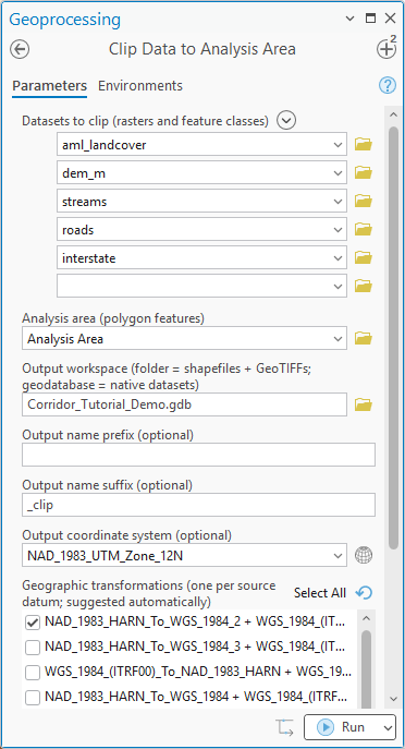
_clip suffix.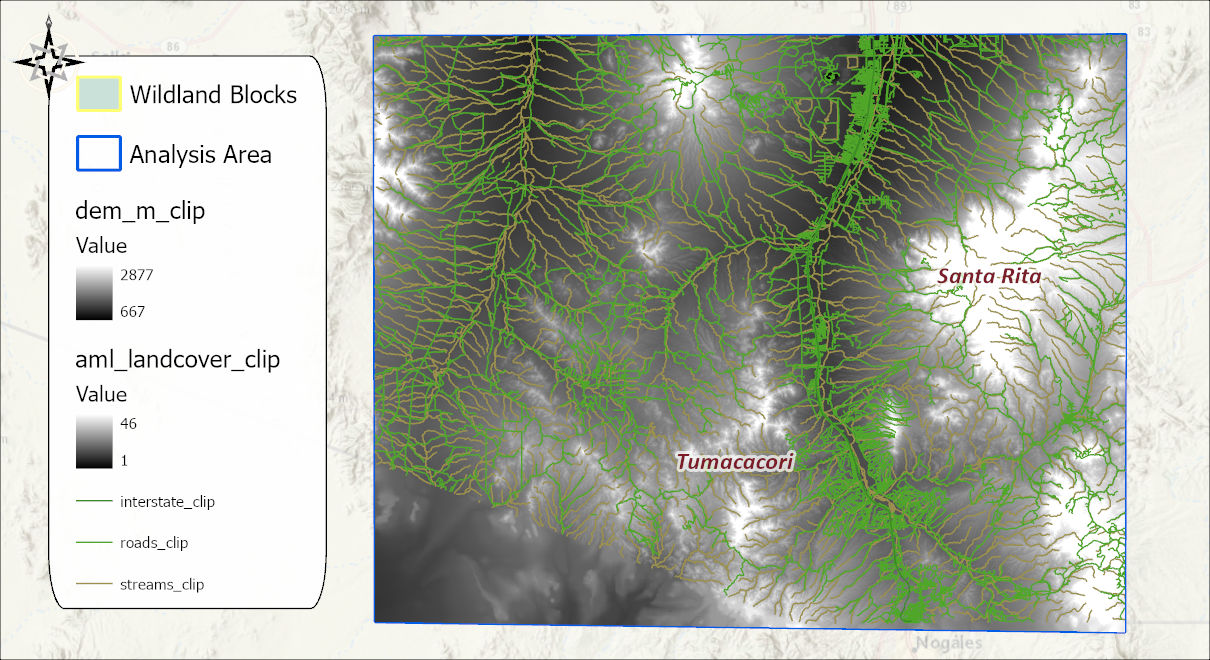
The clip run is also the moment to get every dataset into the same coordinate system. The dialog's optional output coordinate system (NAD 1983 UTM Zone 12N here) projects each clipped dataset on the way out, and when an input sits on a different datum the tool lists the geographic transformations Pro suggests for that datum pair, one per source datum, so you can pick the right one rather than discover the mismatch as a half-pixel shift three steps later. One more caution: each raster keeps its own cell size and grid unless you set the Cell Size and Snap Raster environments on the Environments tab, so set both to the DEM when your rasters do not already share a grid. The tutorial data already share one, which is why the dialog above leaves them alone. The tool's page spells out both routes.
Step 3: Derive the topographic factors
Black bear's habitat model uses four factors: land cover, elevation, topographic position, and distance from roads. These are simply the factors we judged might matter to black bear in this landscape — no law says a model must use exactly these four. A riparian obligate would want distance to water, a desert tortoise would want soils, and a species with good telemetry data might justify a factor you would never think to ask an expert about. Two of the four in our example must be derived:
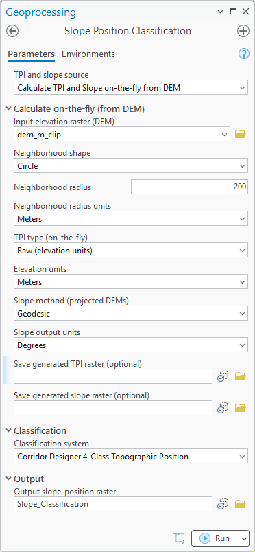
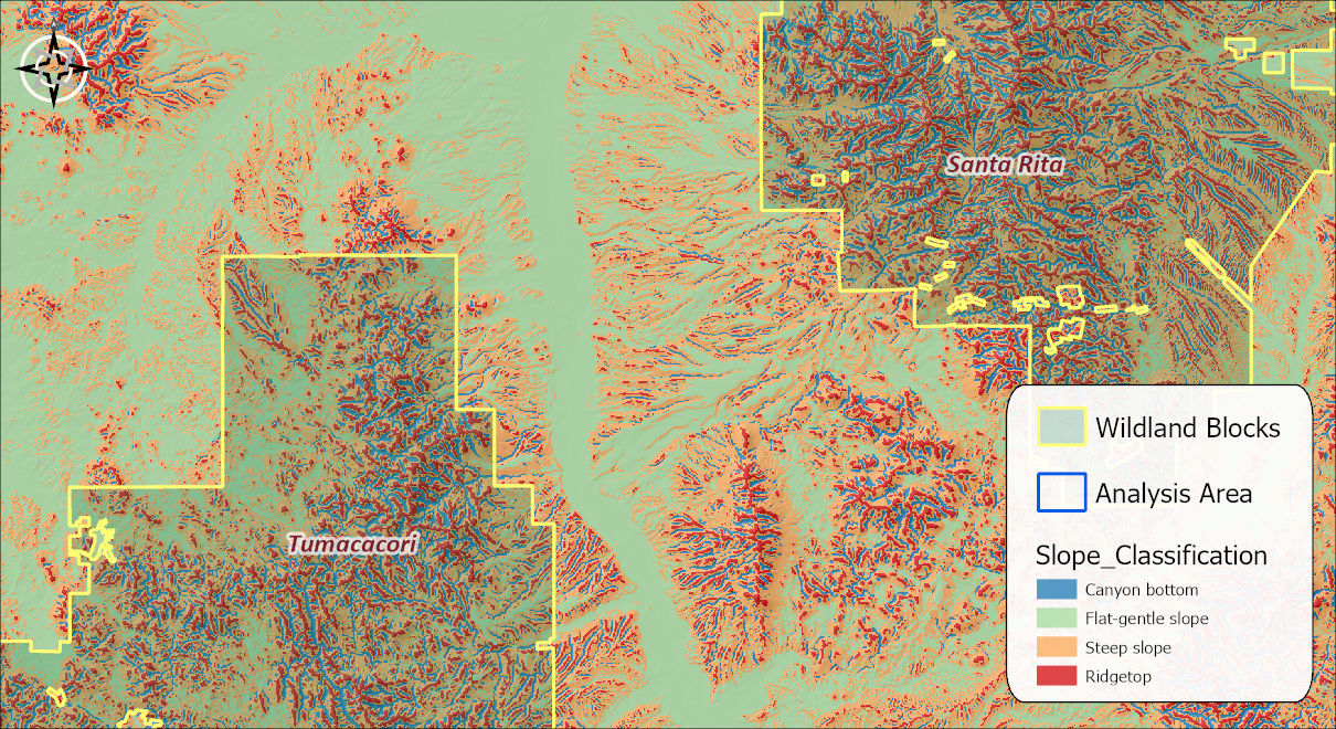
Topographic position. Use the Slope Position Classification tool (in the TPI Tools of the Topographic Analysis group) on the clipped DEM. The Arizona Missing Linkages parameterization, reproduced by this tool's defaults, compares each pixel to the mean elevation within a 200-m radius: at least 12 m below the neighborhood mean is a canyon bottom; at least 12 m above is a ridgetop; otherwise a flat-gentle slope below 6° of slope or a steep slope above it. That particular set of rules ships with the add-in as a saved, named classification system, Corridor Designer 4-Class Topographic Position, so you simply pick it from the Classification system list. If your species or terrain calls for different thresholds, more classes, or other names and colors, the Classification System Builder tool lets you author your own system once and reuse it by name in every classification tool. Drape the result over a hillshade (the Cartography tools' Enhanced Hillshade serves nicely) and judge how well the four classes match the terrain you know.
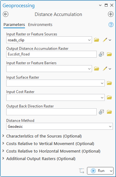
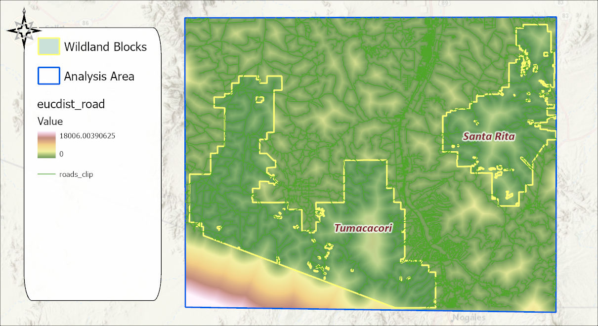
Distance from roads. The fourth factor is a raster
of straight-line distance from the nearest road. This is the
one step of the original chain the add-in does not duplicate:
most projects already have a distance surface or a license to
make one, and we aren't trying to exactly replicate any
existing ArcGIS Pro tools in this add-in. Use whatever
tool you would normally reach for to calculate Euclidean
distance. In this example we use ArcGIS Pro's
Distance Accumulation tool (Spatial Analyst): the
clipped roads are the input source, the distance method is
Geodesic, and every other parameter is left blank. The part
that matters is on the Environments tab: set the
Cell Size, Extent and Snap Raster to the
clipped DEM, so the distance raster lines up with the DEM cell
for cell. Every factor in the model must share one grid, and
this is the step where a mismatch would creep in. Name the
output eucdist_road.
Step 4: Enter the species' suitability scores
We now have the four factor rasters: land cover
(aml_landcover_clip), elevation
(dem_m_clip), topographic position
(Slope_Classification) and distance from roads
(eucdist_road). Each has to be translated into
the species' terms — a suitability score from 0
(non-habitat) to 100 (best) for every class or range of values
it contains. The original toolkit read those scores from
tab-delimited text files, one per factor, prepared by hand
from a species expert's scoring spreadsheet. The Pro add-in
replaces the hand-edited files with the
Create HSM Remap
Table window, which shows you the raster's actual
distribution while you score it and saves the result as a
geodatabase table the modeling tool reads directly.
This is a ribbon window rather than a geoprocessing tool, and
it is the ribbon interface we show in this tutorial; there is no
geoprocessing-pane version of it. You do not need one for
automation, though: the
Create Habitat
Suitability Model tool in the next step accepts either the
saved geodatabase tables or the tab-delimited text
templates directly, so a ModelBuilder or Python workflow can
point at the speciesData text files and skip the
window altogether. Open the window from the Corridor Designer
group of the ribbon and work through the four rasters one at a
time:
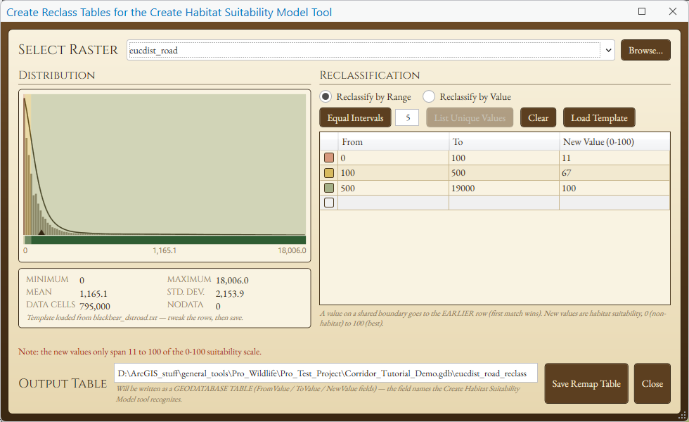
- Select the raster. Pick it from the list of rasters in the map (or browse to it). The window draws its histogram and reports the minimum, maximum, mean, standard deviation and cell counts — so you can see, before scoring anything, that elevation here runs from 667 to 2,877 m and that distance from roads is heavily piled up near zero.
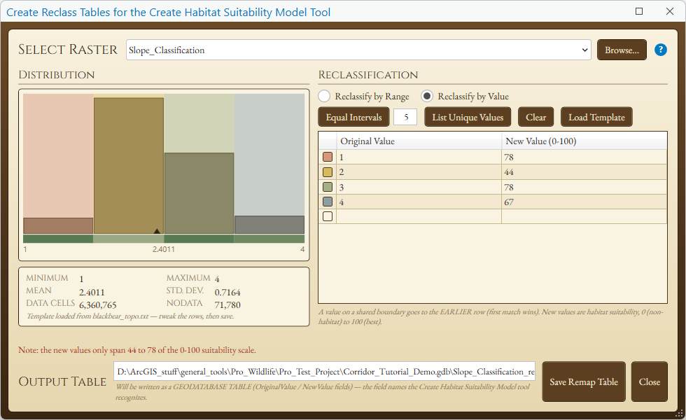
- Choose the reclassification style. Continuous rasters (elevation, distance) are scored by range: each row is a From–To span and its score. Categorical rasters (land cover, topographic position) are scored by value: one row per class code. Equal Intervals splits the range into a chosen number of even bins and List Unique Values lists every class present, either of which gives you a grid to fill in from scratch.
- Or load a template. Load Template reads a
text file in the original toolkit's format —
from to : scorefor ranges,value : scorefor classes — and fills the grid. The sample data'sspeciesData\blackbear\folder holds one for each of the four factors:blackbear_elev_m.txt,blackbear_lndcvr.txt,blackbear_topo.txtandblackbear_dstroad.txt(and the neighboring species folders hold the same four files for eleven other species). Load the one that matches the raster, then edit any row you disagree with. For your own species you will build these grids from your expert's spreadsheet; for black bear the scores translate directly, and the reasoning behind every one of them is in the black bear account of the toolbox documentation. The distance-from-roads factor, for instance, reads: 0–100 m from a road scores 11, 100–500 m scores 67, beyond 500 m scores 100. - Check the coverage. Continuous ranges must span everything in your analysis area — the elevation template runs to 4,000 m and the distance template to 15,000 m for exactly this reason (this area's distances reach 18 km, so that last row is stretched to 19,000 in the figure below). The window also notes when a factor's scores never reach 0 or 100: black bear's elevation scores only span 22 to 100, which simply says that no elevation in this landscape is outright non-habitat for a bear.
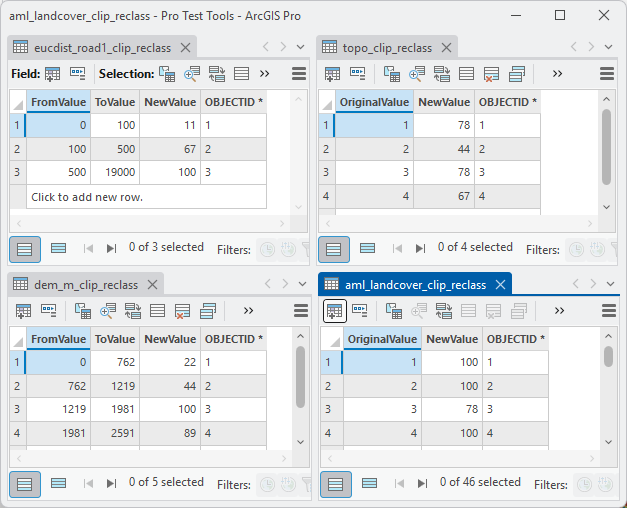
- Save the remap table. Set the output table's name and location (the project geodatabase) and click Save Remap Table. A range table carries FromValue, ToValue and NewValue fields; a value table carries OriginalValue and NewValue — the field names the Create Habitat Suitability Model tool recognizes.
When you score land cover, keep the
Ancillary_Files folder open: aml_landcover.xls
names each of the 46 codes and the vegetation description
appendix describes them, which is how the expert decided that
ponderosa pine forest earns 100 and agricultural or urban
classes earn 0.
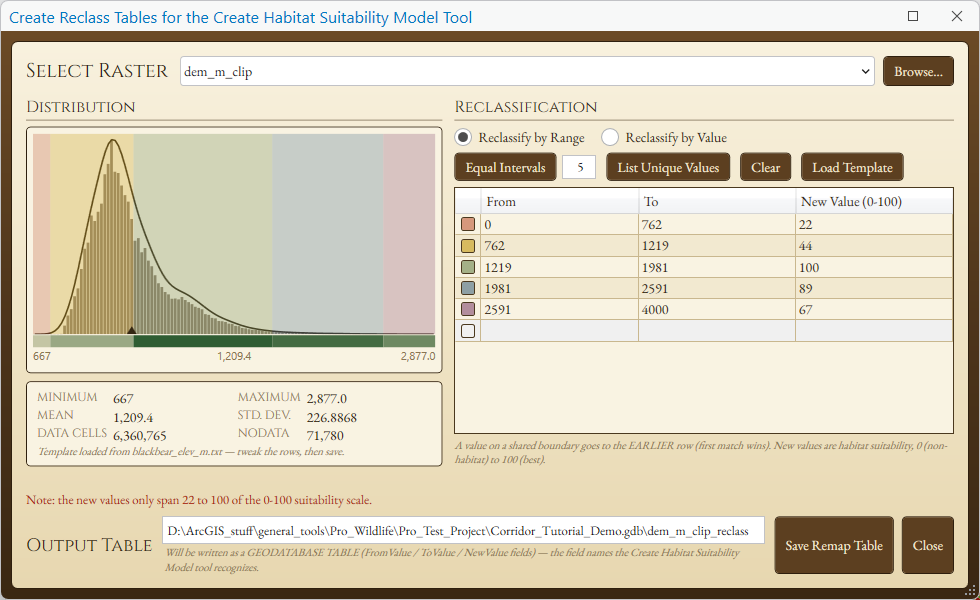
blackbear_elev_m.txt template: mid elevations
score 100, the lowest desert 22.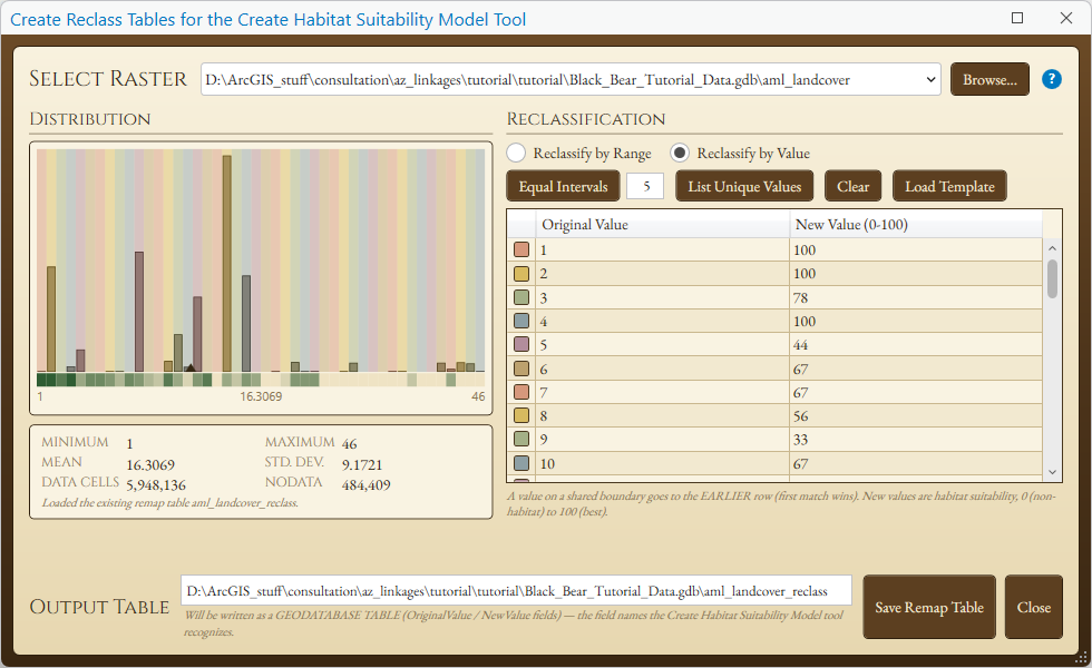
Step 5: Create the habitat suitability model
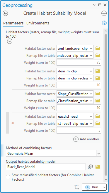
Run Create Habitat Suitability Model. Each row of the dialog is one habitat factor: the factor raster, the remap table that scores it, and its weight. Enter the four factors, each paired with the remap table you just saved for it in Step 4:
| Habitat factor raster | Remap table | Weight |
|---|---|---|
aml_landcover_clip | aml_landcover_clip_reclass | 75 |
dem_m_clip | dem_m_clip_reclass | 10 |
Slope_Classification | Slope_Classification_reclass | 10 |
eucdist_road | eucdist_road_reclass | 5 |
The weights are the expert's judgment of how much each factor
matters to black bear, and they must sum to 100. Land cover
carries three quarters of the model: for a bear, what grows on
the ground — oak woodland, pine forest, chaparral —
matters far more than anything else. Elevation and topographic
position get 10 each, mostly as proxies for the same vegetation
and for cover, and distance from roads gets 5. These are the
numbers in blackbear_weights.txt, and the black bear
account in the toolbox
documentation explains the thinking behind them. For your own
species, the weights are as much a part of the expert's model as
the scores are, and just as worth arguing over.
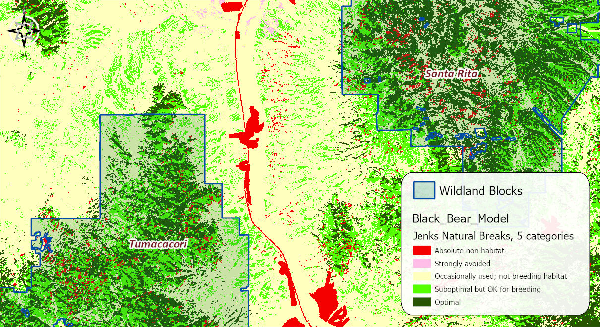
Then choose the method of combining factors. The tutorial uses the geometric mean, which lets a very poor score on any one factor drag the pixel down toward it — usually the right behavior for limiting factors, since a bear does not average its way across a freeway. The additive (weighted arithmetic) mean is the gentler alternative, and comparing the two on the same landscape is a worthwhile detour. Name the output and run. The result is the 0–100 suitability surface for black bear, delivered with the add-in's ready-made symbology: five natural-breaks classes labeled with the same biological anchors the About Corridor Design page describes, from absolute non-habitat to optimal.
A word about those five classes. The breaks come from Jenks natural breaks, which is a reasonable way to cut a 0–100 surface into five groups: it looks for the gaps in the distribution of values and places the breaks there. But it is a numeric clustering method, nothing more. It knows nothing about bears, and it was not designed to find the five habitat classes the labels name; it simply happens to work well here as a draft classification. Treat the breakpoints as a starting point. If your expert says that anything below 30 is non-habitat for this species, or that breeding habitat starts at 60, open the layer's symbology and move the breaks to those values.
Step 6: Map the habitat patches
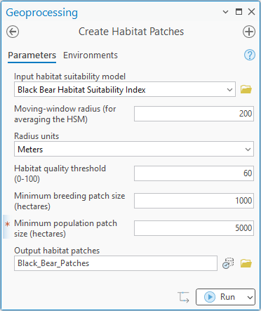
Run Create Habitat Patches on the suitability model. We identify patches and rank their ecological importance based on three parameters: the suitability surface is first averaged in a moving window matched to what we think might be the species' perceptual range (a 200-m radius circle for black bear — and mind the units: 200 meters, not 200 cells); pixels above the quality threshold (60, matching the Arizona Missing Linkages standard) become candidate habitat; and contiguous habitat areas are classed by size — at least 1,000 ha makes a potential breeding patch, at least 5,000 ha a potential population patch (the Pro tool computes the areas geodesically). The output classes — population patch, breeding patch, smaller-than-breeding — arrive symbolized and become the raw material for corridor termini.
blackbear_patches.txt.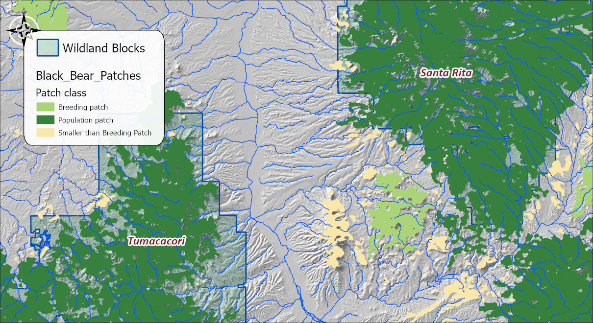
Step 7: Model the corridor
Three tools replace the original monolithic corridor step, and make its internals visible: one finds the endpoints, one turns suitability into travel cost, and one builds the corridor.
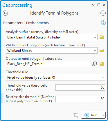
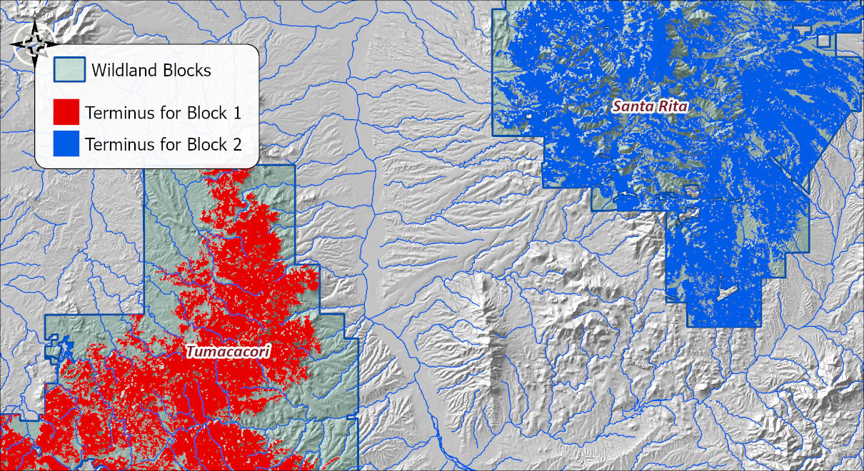
Identify Termini Polygons finds the corridor's start and end points inside each wildland block: the concentrations of good habitat the corridor should connect. Give it the black bear suitability model and the wildland block polygons. Inside each block it keeps the cells above a threshold — use the Fixed value rule with 60, the same quality threshold the patch map used, so the termini are the block's habitat-quality cores — and groups them into contiguous regions. Inside a block those regions come in every size, from one large mass of good habitat down to specks of a cell or two, and the relative size threshold decides which of them are big enough to count as termini. Be clear about what the percentage is measured against: it is not a share of the wildland block. It is a share of the largest contiguous region in that block. The tool finds the biggest region of above-threshold cells in each block, and a region is kept only if it is at least that percentage of the biggest one's size. So at 50% only the largest region and any others at least half its size survive as candidate start and end points; in practice, for a block with one dominant mass of habitat like these two, that means the one big region and nothing else, which is the Pro equivalent of the original's rule of starting from the population patch. At 100% only the single largest region survives; at 0% every region is kept, down to the specks. Leave it at 50% for black bear. Lowering it toward 0% would keep every fragment above 60 as a terminus, and because the corridor tool treats all of a block's termini as one set of starting cells, a fragment sitting at the block's edge would hand the corridor a cheap starting point right at the boundary — exactly the “room to run” problem the About page warns about. The honest caveat from the original still applies: if a block holds no real concentration of good habitat at all, a corridor model for this species deserves a rethink.
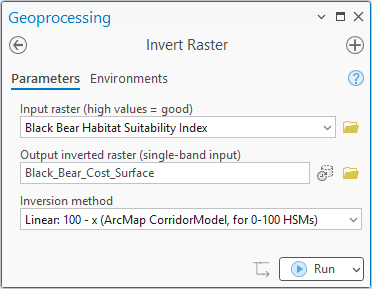
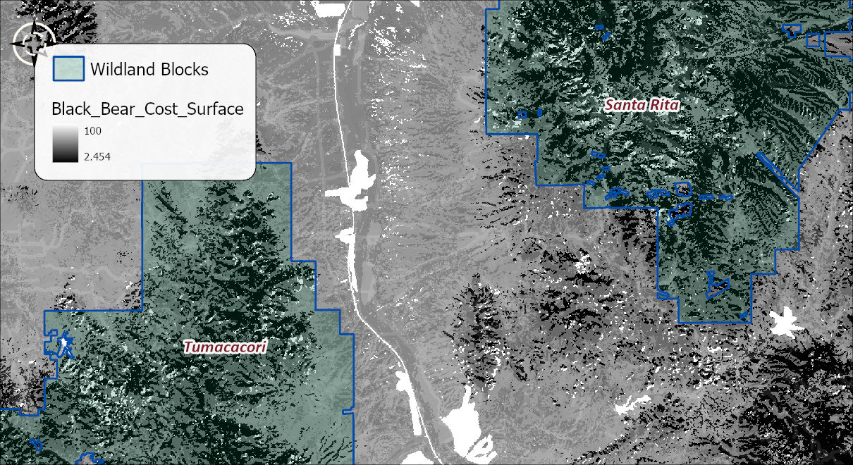
Invert Raster turns
the suitability model into the cost surface the corridor
tool needs. A least-cost analysis wants low values to mean easy
travel, and our model is the other way round: 100 is the best
habitat. The original CorridorModel tool made this flip
internally, as resistance = 100 − suitability;
the Pro tools make it a visible step, so that the cost surface
is a real raster you can inspect, and so that the corridor tool
can also accept cost surfaces that arrive already pointing the
right way, such as the Land Facet Mahalanobis distances. Run
Invert Raster on the black bear model, choose the Linear:
100 − x method — the exact conversion
the ArcMap tool applied, so your corridor is comparable with one
built there — and name the output something like
Black_Bear_Cost_Surface. The default Reciprocal method,
1/(x + c), is the other legitimate choice; it punishes
poor habitat far more harshly, and the
Invert Raster page
explains how differently the two route a corridor. Whichever you
pick, check the result once: the interstate and the town should
now be the highest values on the map, and consequently
the most expensive for the animal to cross.
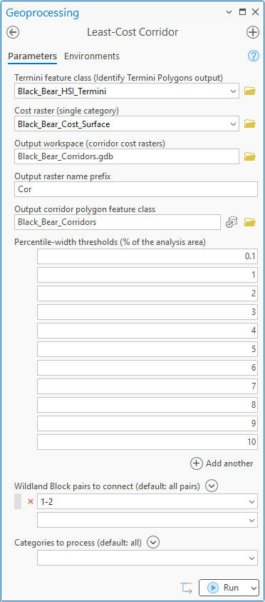
Least-Cost Corridor then takes the termini feature class and the cost surface, accumulates cost-distance from the termini in both blocks, sums the two surfaces, and slices the result. Slices are expressed as the most permeable percentage of the landscape — the 0.1% slice is the skinny spine of the corridor, the 3% slice a broad swath, and the nested set from 0.1% to 10% lets you watch the corridor widen and sprout strands as the threshold loosens. Choosing the slice to carry forward is a biological judgment, not a mechanical one: wider than a home-range width for corridor-dwelling species, against the practical limits of what can be conserved (see the discussion on the About page).
The dialog has two optional lists at the bottom worth a
word. Wildland Block pairs to connect lets you build
corridors between only the pairs you name. The entry in the
figure, 1–2, is there purely to illustrate the parameter:
this example has only two blocks, so leaving the list empty
would have built the same single corridor. With three or more
blocks the list matters, because by default the tool builds a
corridor for every pair. The block numbers it offers are not
typed in; they come from the Block attribute field
of the termini feature class, which Identify Termini Polygons
creates for exactly this purpose, so the dropdown shows the
pairs that actually exist. Categories to process is for
land facet runs, where one termini feature class carries
several facets; a single-species run has one category and the
list can stay empty.
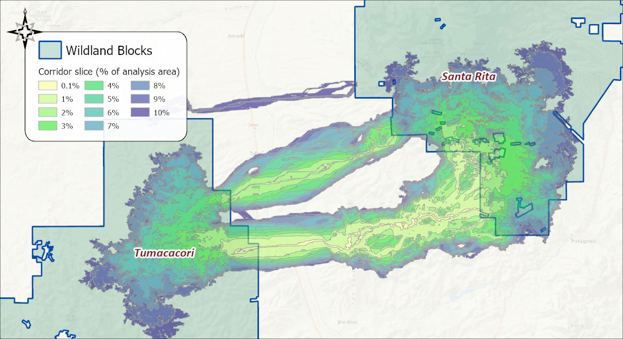
Read the picture the way the book asks. The spine is the single cheapest route; each wider slice adds the next-cheapest ground around it. The strands show what “sprouts additional strands” means. The second band, looping north of the main one, is not part of the corridor at 1% or 2%, but by 5% the model has found that second way across, and it stays a distinct band of its own all the way to 10%, joined to the main band only by a thin 10% connector. And at about 9% a third, much narrower strand appears farther north still. So the widest slice is not one broad corridor but three routes of very different quality, and a reader deciding which slice to carry forward is also deciding how many of those routes to keep. That is the biological judgment discussed above; the picture is what makes it an informed one.
Step 8: From one corridor to a linkage
The black bear corridor is one species' answer. A real linkage design repeats Steps 4–7 for every focal species and combines the results, and the reason is not thoroughness for its own sake. A single-species corridor embodies one set of expert scores, one body size, one way of moving through the landscape; defend it and you are defending that one species' ecological requirements, and every other species is served only by accident. A multi-species design is more ecologically defensible than any single-species design because each species is, in effect, a different instrument reading the same landscape: a bear reads forest and distance from roads, a jackrabbit reads open grassland, a rattlesnake reads slope position and temperature. Ground that several of them select is ground that works for several kinds of life, and ground that only one selects is still ground that species needs. The union of the corridors is the linkage; the differences among them are the argument for it.
The sample data carries scores, weights and patch parameters
for eleven more species from the same workshops, in
speciesData\, one folder each. Run the chain for
all of them — the same wildland blocks, the same factor
rasters, the same 2% slice, so that no species gets more ground
than another by construction — and twelve corridors come
out. Each map below shows one species' corridor in orange with
the other eleven in gray behind it.
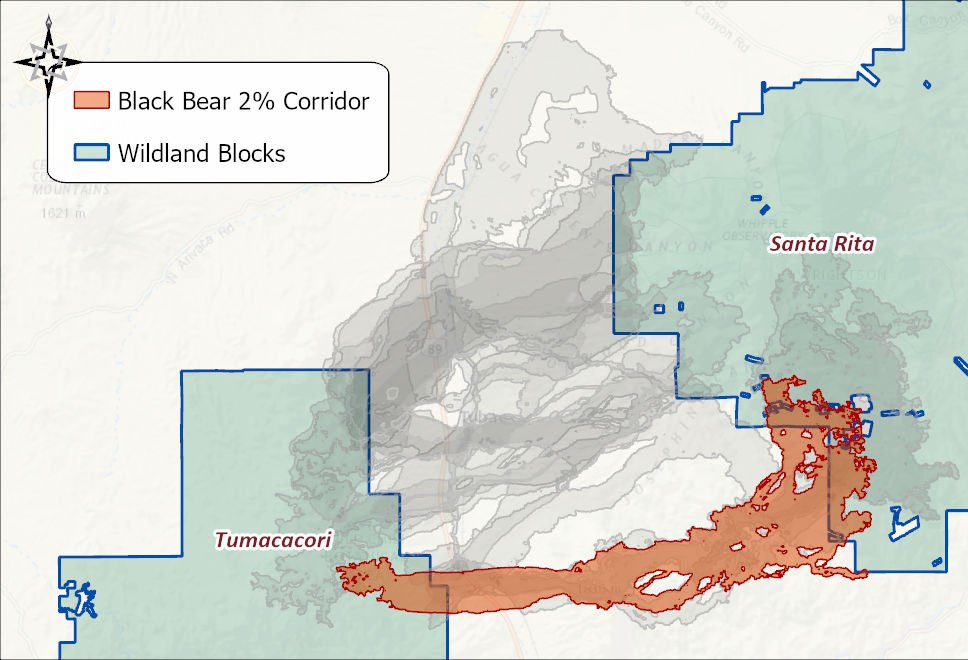
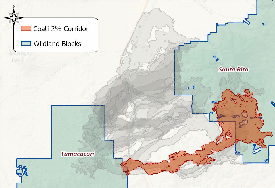
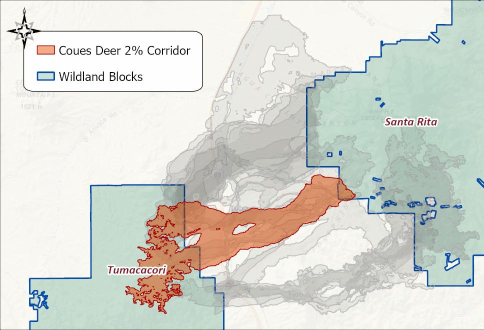
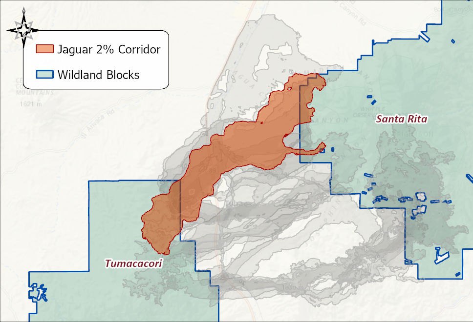
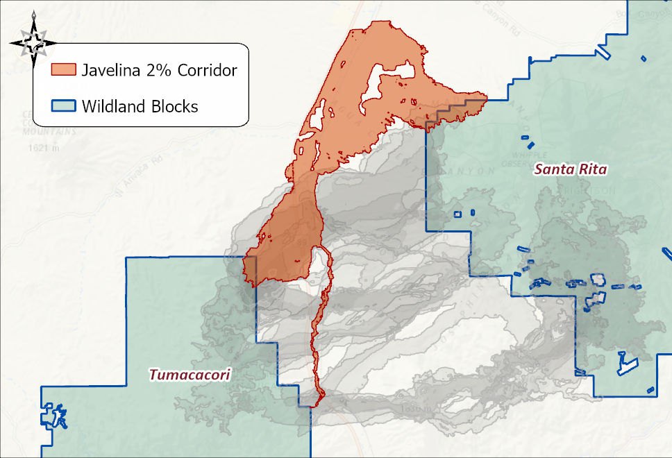
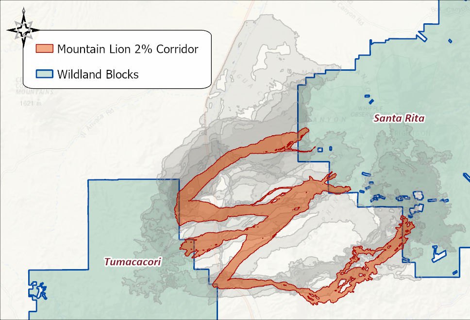
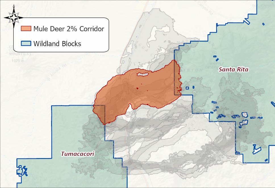
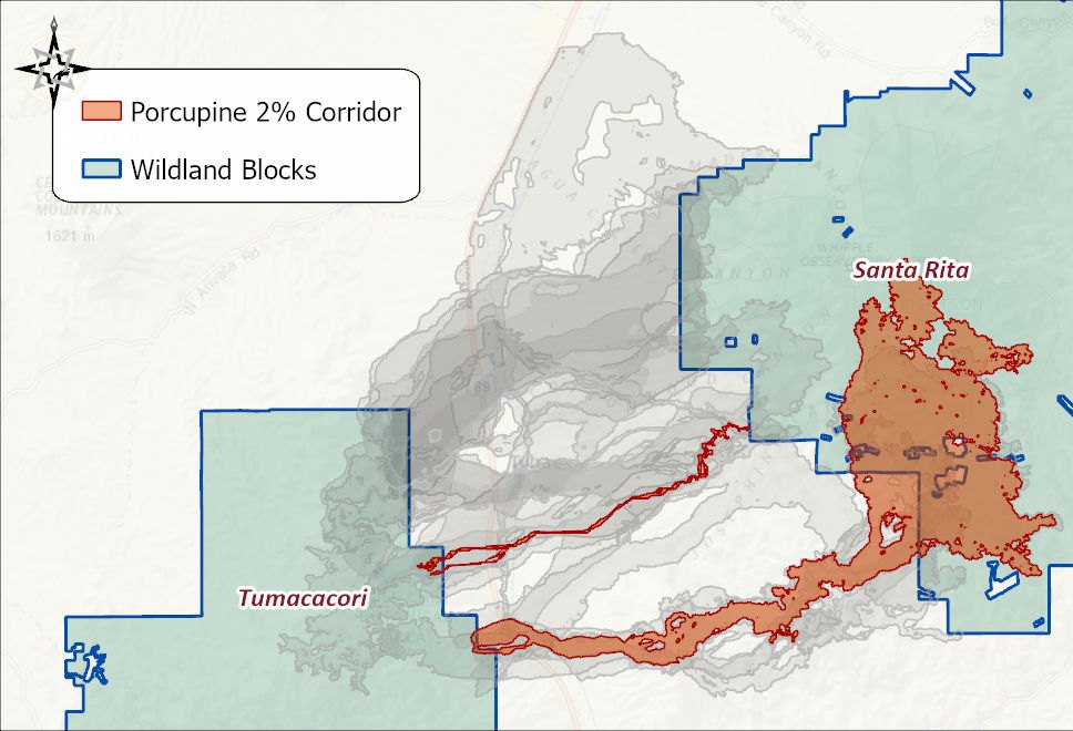
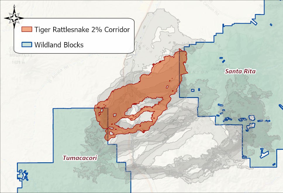
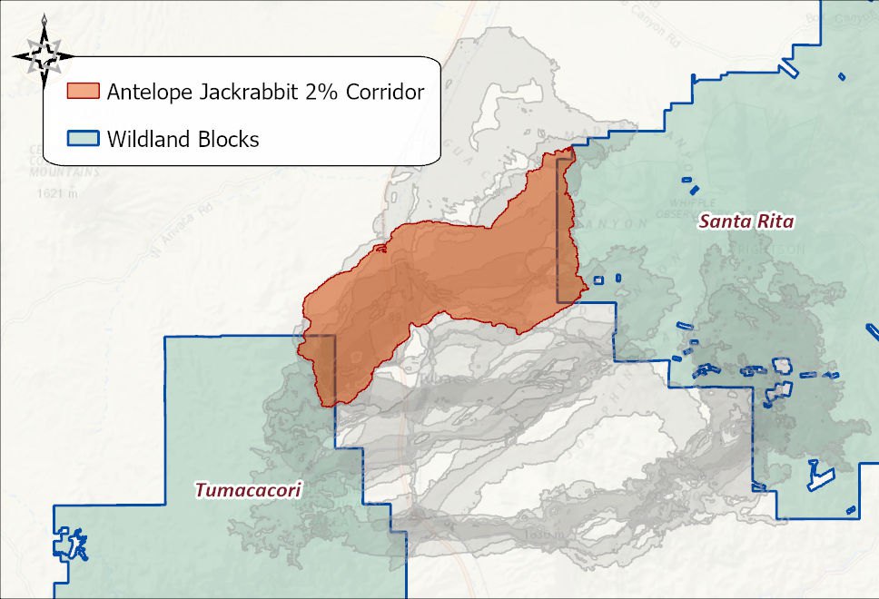
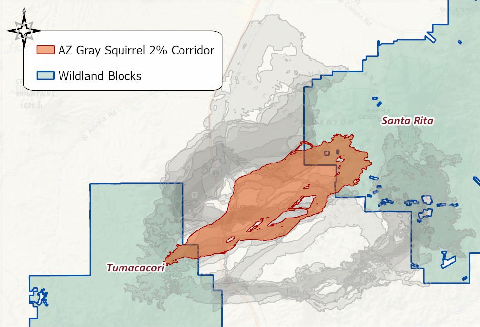
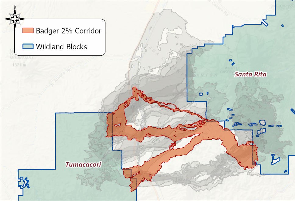
Look at the maps as a set and the landscape sorts itself. The forest and woodland animals — bear, coati, porcupine, gray squirrel — hold to the southern route along the Tumacacori highlands and spill into the Santa Rita foothills. The open-country animals — jackrabbit, mule deer, javelina, rattlesnake — swing north through the valley grasslands. The wide-ranging carnivores hedge: the mountain lion's corridor is three strands, the badger's a loop, and the jaguar keeps to the northern flank of the valley and enters the Santa Rita block at its northwest corner. No single one of these is the linkage. Together they are.
Union the corridors
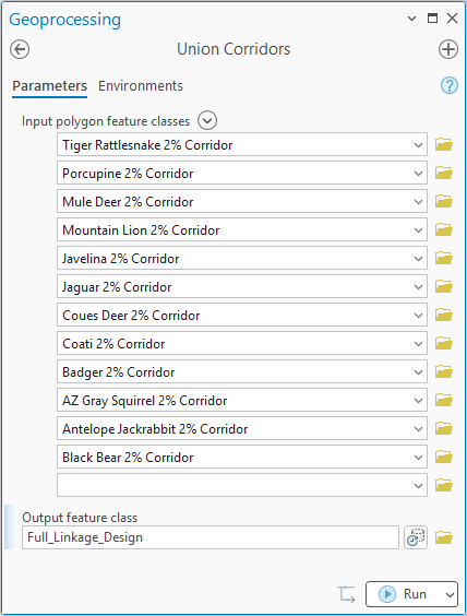
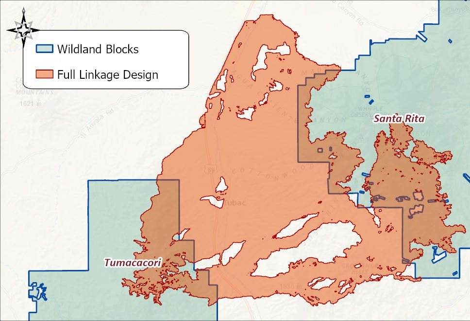
Union Corridors takes the twelve corridor feature classes and returns one seamless polygon: unioned, then dissolved, so the result answers “is this ground part of any corridor?” and nothing else. Attributes are deliberately dropped — which species wanted a piece of ground is the next tool's job.
Fill the holes that do not mean anything
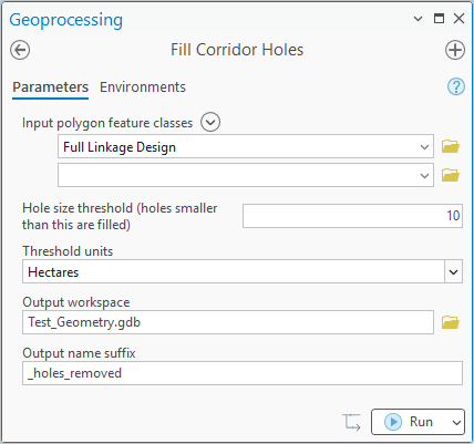
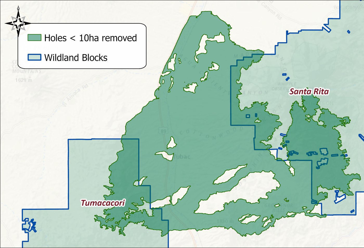
The union is full of holes, and they are not all the same kind. Most of the small ones are artifacts of slicing — a percentile threshold crossing a knoll, a cost surface a few points too high on one side of a wash — and a linkage design drawn around them would be a design nobody could implement. The large ones may be real: a town, an interstate, a block of converted land that genuinely is not linkage. Fill Corridor Holes lets you set the line between the two. Here every hole under 10 hectares is filled, in one pass, and anything larger is kept for a closer look.
Where the species agree
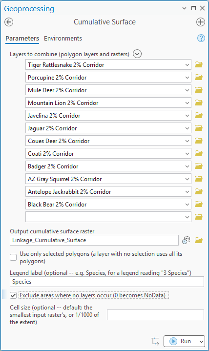
The union says where the linkage is; it cannot say which parts of it matter most. Cumulative Surface answers that by stacking the twelve corridors and counting, cell by cell, how many of them cover each spot. The result is a raster from 1 to 12 (here the maximum reached is 8), with a legend that reads directly as “3 Species”, “7 Species”.
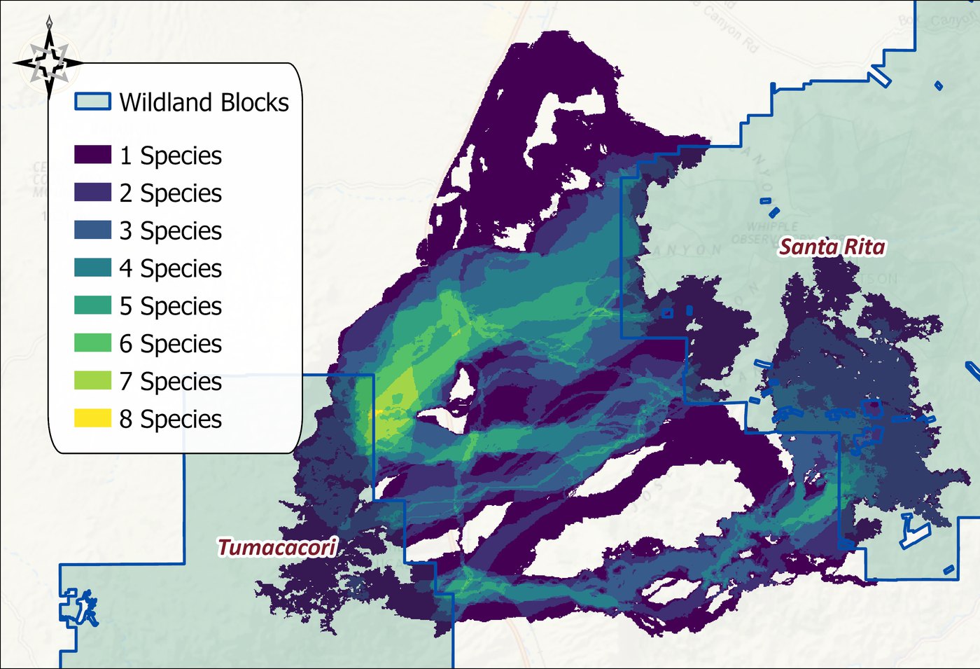
The bright ground is where the species agree, and agreement among twelve independently scored models is strong evidence that a piece of land is important to a great many kinds of animals — a natural place to begin conservation, and a persuasive map to put in front of a landowner or a county board. But read the dark ground carefully too. A cell that only one species chose is not a cell to give up; it may be the only way a jaguar gets through, and a species that is critically endangered, or that the project exists to serve, may deserve far more weight than one vote in twelve. The count is a starting point for a judgment, not a substitute for it.
A record of the whole analysis: the Corridor Analysis Data Report
One more thing, and it applies to every Corridor Designer tool, not just the linkage steps. Every output in this chain carries provenance metadata, written by the tool that made it, and the Corridor Analysis Data Report window reads it back as a plain-language account of how any dataset in the project came to be. Pick the corridor feature class in the window and click Describe:
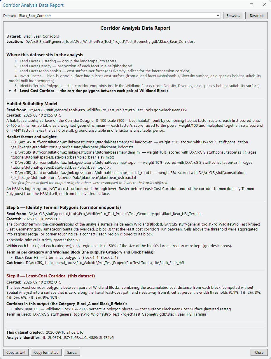
What it is showing is the corridor's entire ancestry, recovered from metadata rather than from memory. The outline at the top places the dataset in the chain: this is step 6, Least-Cost Corridor. The Habitat Suitability Model section then lists the four factor rasters with their weights (75, 10, 10, 5) and the remap file each was scored with, and states the combining rule in words: a weighted geometric mean, each factor's score raised to the power weight/100 and multiplied together, so a zero in any factor makes the cell zero. The Identify Termini section records the wildland blocks, the threshold rule (cells strictly greater than 60) and the relative size rule (regions at least 50% of the block's largest), and reports that it produced two termini, one per block. The Least-Cost Corridor section names the cost surface it walked, flags it as an inverted raster, lists the eleven percentile thresholds, and counts the sixteen polygon pieces that came out. Each section carries the source dataset's path and creation time, and the report ends with an analysis identifier shared by every dataset in the run.
This is the answer to a question every corridor project eventually faces: six months later, which suitability model, which weights and which threshold produced this corridor? With the original tools the honest answer was often a guess from file names. Here it is one click, it is written by the tools themselves so it cannot drift from what was actually run, and the Copy and Save buttons drop it straight into a report or an appendix.
Recommended citation
Credits and references
Tutorial adapted from Chapter 6 of the workshop book; the tutorial dataset and black bear parameterization are from the Arizona Missing Linkages project, funded by the Arizona Game and Fish Department.
- Beier, P., D. Majka, and J. Jenness. 2007, revised 2026. Designing wildlife corridors with ArcGIS: ArcGIS Pro edition. Workshop book, revised by J. Jenness for the Corridor Designer Tools of the Wildlife and Forestry Tools add-in. Available at: CorridorDesigner_WorkshopBook_2026_ArcGISPro.pdf (5 MB)
- Beier, P., D. Majka, and J. Jenness. 2007. Designing wildlife corridors with ArcGIS. Workshop book, Northern Arizona University. Available at: corridordesign.org (archived copy at the Internet Archive)
- Majka, D., J. Jenness, and P. Beier. 2007. CorridorDesigner: ArcGIS tools for designing and evaluating corridors. Available at: corridordesign.org (archived copy at the Internet Archive)
Related tools and pages
- About Corridor Design — the concepts behind every step here.
- About Land Facet Corridors — the climate-change-robust alternative workflow, with its own tutorial.
- The individual tool pages (Create Habitat Suitability Model, Create Habitat Patches, Identify Termini Polygons, Least-Cost Corridor, and the rest) as they come online — the sidebar tracks the full set.