

Diversity Indices
Summary
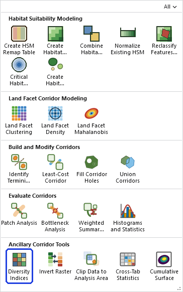
Measures the neighborhood diversity of a categorical raster — each cell of the output describes how diverse the species, community, or category values are within a moving neighborhood around that cell. Choose among the major diversity measures: the effective number of species (Hill numbers, with a selectable order q — the default, and the most interpretable: the number of equally common categories that would give the same diversity), Shannon's index, the Gini-Simpson index, and Simpson's concentration (a dominance measure, where higher means less diverse). A raster whose attribute table carries more than one classification can be measured by any of them: choose the attribute field, and the cells are classified by that field's values before the diversity is computed. Neighborhoods may be rectangles, circles, annuli, wedges, or custom kernel files, with geodesic handling for geographic-coordinate rasters. A modernized, generalized port of the Land Facet Corridor Designer's ArcMap Shannon's Index tool; no Spatial Analyst needed.
Beyond corridor work, a diversity raster is a useful way to fold a categorical dataset into analyses that need continuous variables — for example, as a landscape variable in a Mahalanobis distance analysis, following Clark et al. (1993), who used exactly this kind of neighborhood-diversity derivative of their vegetation map.
In the Land Facet chain
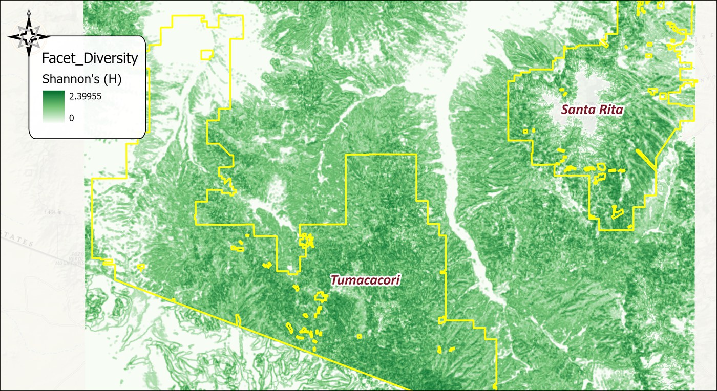
Run on a land facet raster, Shannon's H′ is the interspersion surface of the Land Facet workflow: invert it with Invert Raster (reproducing the published 1/(H′ + 0.1) resistance) and model the facet-diversity corridor on the result.
A tour of the dialog
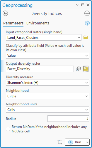
The example is Step 5 of the Land Facet Tutorial: the diversity of eighteen land facets in a 5-cell circle, measured with Shannon's index to follow the published method. The tool's default measure is the effective number of species, which is exp(H) at order 1 and ranks the landscape identically; the tutorial chooses Shannon's H so that the 1/(H′ + 0.1) resistance of the original work can be reproduced exactly.
Classifying by an attribute field
A categorical raster often carries more than one
classification in its attribute table. The tutorial's land
cover raster has 26 vegetation types in its Value column and,
beside them, a Vegetation column naming them and an
NLCD column grouping them into 10 broader classes;
a Landfire EVT raster carries several such systems. The
Classify by attribute field list offers Value, the
default, under which every distinct cell value is its own
class, plus every text or integer column of the attribute
table. Choose a column and every cell is relabeled by it before
the neighborhood counting, so the diversity is measured over
that column's classes: the 10 NLCD groups rather than the 26
vegetation types. Cells sharing an entry become one class, a
blank entry is its own class, and a cell value with no row in
the table keeps a class of its own, with a warning. A raster
without an attribute table offers only Value, and the list is
disabled. This is the same regrouping the
Cross-Tab Statistics
window offers for its raster variables.
One caution for a land facet raster: keep Value. The
facet is the cell value. Its attribute table also carries a
Category column, which groups the facets by their
first-pass class, four classes instead of eighteen, and a
Cluster column, which is only the cluster number
within each category. Classifying by Cluster merges unrelated
facets, canyon-bottom cluster 1 with ridgetop cluster 1, into
classes that mean nothing.
The example in the next section shows the option at work: the tutorial land cover raster classified by its NLCD column, with the dialog and the before and after maps.
The tool holds the whole raster in memory at once, so the memory it needs grows with the number of cells. On most rasters that is no concern. On a very large one the tool may need more memory than your computer has free, and then one of two things happens: Windows starts using the disk as overflow memory and the tool slows to a crawl, or the tool stops with an out-of-memory error. There is no fixed limit; it depends on how much memory your computer has free. If a raster is too large, clip it to the area you need first.
Why the effective number of species
Shannon's index has been the workhorse of diversity measurement since the 1940s, and it is still the right choice when a published method calls for it, as the land facet method does above. But the tool's default measure is the effective number of species, and the reason it has been gaining ground on the traditional indices is that it answers the question people actually ask. Shannon's H′ is measured in bits or nats of uncertainty; the Gini-Simpson index is a probability that two draws differ. Neither is a number of anything. The effective number is: it is the number of equally common categories that would give the same diversity, so a value of 4 means the neighborhood is as diverse as one holding four categories in equal shares, and a value of 12.7 means the equivalent of nearly thirteen.
That interpretability comes with a property the traditional indices lack, which Jost (2006) called the replication principle: double the diversity, in the sense of two equally diverse, non-overlapping communities put together, and the effective number doubles. Shannon's H′ rises by only 0.69 no matter how diverse the halves were, and the Gini-Simpson index, already compressed toward its ceiling of 1, barely moves at all. So a landscape with H′ of 2.0 is not twice as diverse as one with 1.0, and a Gini-Simpson of 0.9 against 0.8 hides a larger difference than it shows, whereas effective numbers of 7.4 and 2.7 mean what they say and can be compared, differenced and put in ratios without apology. This is also why the traditional indices are so hard to explain to a stakeholder, and why a map of effective numbers needs relatively little explanation.
The effective number is not a rival to the older indices so much as a common currency for them. Hill (1973) showed that richness, Shannon's index and Simpson's index are all members of one family, differing only in how much weight they give to rare categories, and that each converts to an effective number of species: richness as it stands, Shannon's H′ through exp(H′), and Simpson's concentration through its inverse. The order q below is that family's dial. Converting every index to the same units makes them comparable with one another, and it makes the choice among them a choice about rare categories rather than about scales.
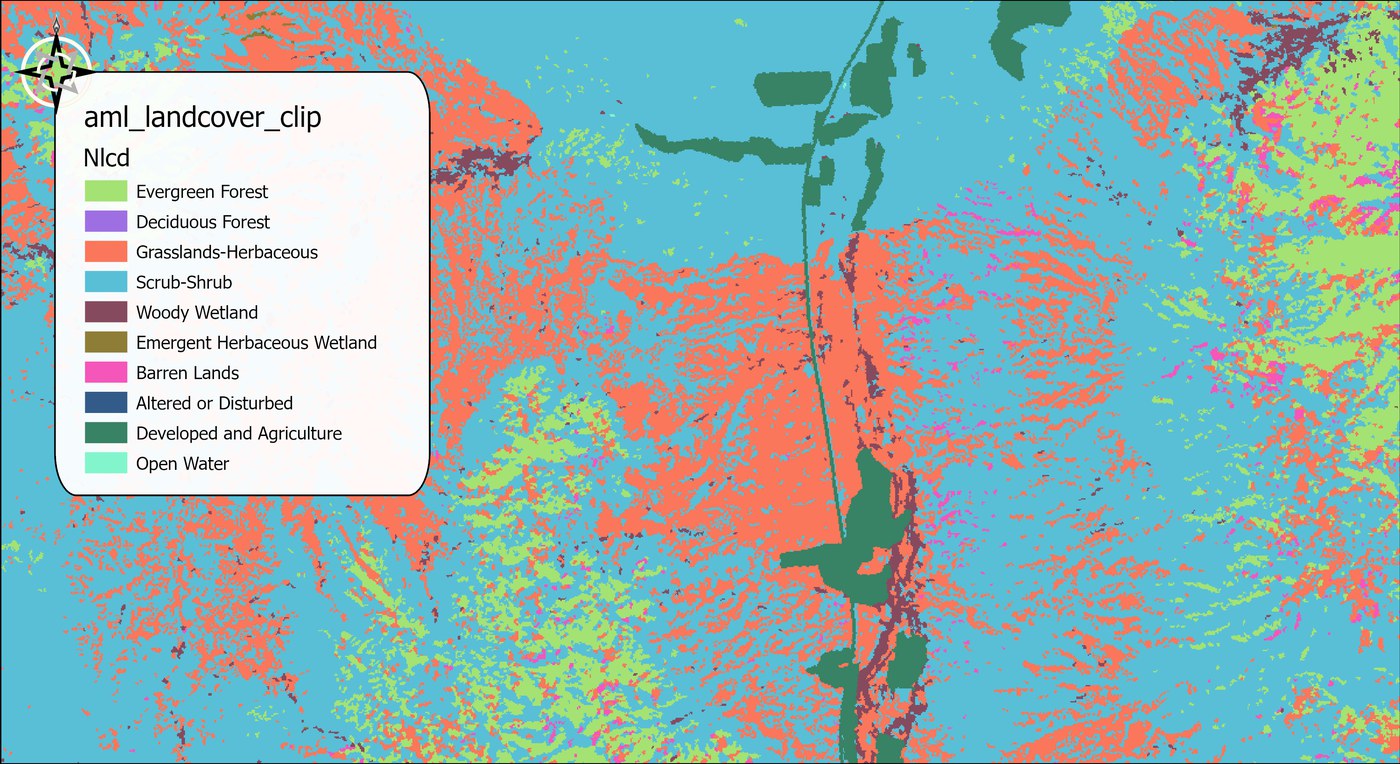
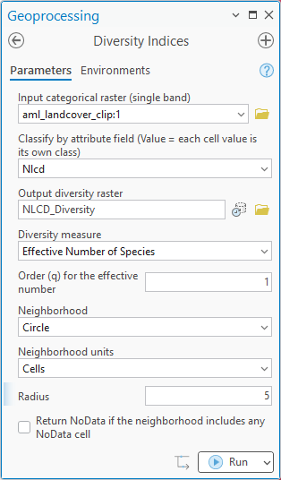
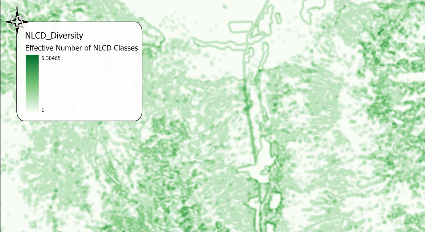
The example below puts both ideas to work on the tutorial's land
cover raster, which carries 26 vegetation types in its Value column
and their 10 NLCD groups in an Nlcd column. The raster
is in the
tutorial data as
aml_landcover (the run below used the copy clipped to
the analysis area), so you can open its attribute table and see
for yourself that it also carries a Vegetation
column, naming each of the 26 types. Classifying by
Nlcd and asking for the effective number of species
gives a map of how many NLCD classes, in equal-share terms,
surround each cell. Classifying by Vegetation instead
would give an entirely different map, because a window that holds
one NLCD class may hold several vegetation types within it: the
same ground, measured at a finer classification, is more
diverse. Which map is the right one depends on which
classification matters to the question you are asking.
The order q, in one paragraph
The effective number of species (Hill numbers) comes with a dial: q = 0 is plain richness (every category counts equally, however rare); q = 1 (the default) weights categories by their abundance (exp of Shannon's H′); q = 2 emphasizes the dominant categories (inverse Simpson). Any q ≥ 0 is allowed, and running several makes a diversity profile. The effective number reads naturally: a value of 3.2 means the neighborhood is as diverse as one with 3.2 equally common categories. (Inverse Simpson is deliberately not a separate menu choice — it is the effective number at q = 2.)
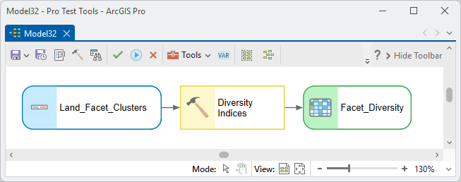
ModelBuilder
Parameters
| Label | Explanation | Data type |
|---|---|---|
| Input categorical raster (single band)Required · in_raster | Each cell a class: a species, community, land-cover or land-facet code. A raster with thousands of distinct values is taken for a continuous one and refused. | Raster Layer |
| Classify by attribute fieldOptional · class_field | Value (default) treats every distinct cell value as its own class; any text or integer column of the raster's attribute table classifies the cells by that column instead. Only Value is offered when the raster has no attribute table. | String |
| Output diversity rasterRequired · out_raster | The continuous diversity surface, symbolized on delivery. A name inside a geodatabase gives a geodatabase raster; a name in a folder gives a GeoTIFF. | Raster Dataset |
| Diversity measureRequired · index | Effective Number of Species (default), Shannon's Index (H), Gini-Simpson Index (1 − D), or Simpson's Concentration (D). | String |
| Order (q) for the effective numberOptional · q | The Hill order: 0 richness, 1 (default) the exponential of Shannon's H, 2 inverse Simpson; any value at or above 0. Used only by the effective number. | Double |
| NeighborhoodRequired · neighborhood | Rectangle, Circle (default), Annulus, Wedge, Irregular or Weight; the last two read a kernel file. | String |
| Neighborhood unitsOptional · nbr_units | Cells (default), Meters, Kilometers, Feet or Miles for the dimensions below; ground units are handled geodesically on a geographic raster. | String |
| Radius, Width, Height, Inner radius, Outer radius, Start angle, End angleOptional | The dimensions of the chosen shape: radius for a circle; width and height for a rectangle; inner and outer radius for an annulus; radius and the two angles (degrees counter-clockwise from east) for a wedge. Only the ones the shape needs are enabled. | Double |
| Kernel fileOptional · kernel_file | A text file of cell weights for the Irregular (any nonzero = in) or Weight (weighted) neighborhood. | File |
| Return NoData if the neighborhood includes any NoData cellOptional · exclude_null | Unchecked (default), NoData cells are simply left out of the neighborhood's count; checked, any NoData cell in the window makes the output NoData. | Boolean |
Python
import arcpy
arcpy.ImportToolbox(r"C:\path\to\JennessEnterprisesTools.pyt")  # your install path
arcpy.jenness.DiversityIndices(
    in_raster=r"D:\tutorial.gdb\aml_landcover_clip",
    class_field="Nlcd",                     # or "Value" for the cell values
    out_raster=r"D:\tutorial.gdb\Effective_Number_NLCD",
    index="Effective Number of Species", q=1,
    neighborhood="Circle", nbr_units="Cells", radius=25)
Recommended citation
Credits and references
By Jeff Jenness, Jenness Enterprises (www.jennessent.com), modernizing the Land Facet Corridor Designer's Shannon's Index tool (Jenness, Brost and Beier).
- Hill, M. O. 1973. Diversity and evenness: a unifying notation and its consequences. Ecology 54:427–432. doi.org/10.2307/1934352
- Jost, L. 2006. Entropy and diversity. Oikos 113:363–375. doi.org/10.1111/j.2006.0030-1299.14714.x
- Shannon, C. E. 1948. A mathematical theory of communication. Bell System Technical Journal 27:379–423. doi.org/10.1002/j.1538-7305.1948.tb01338.x
- Simpson, E. H. 1949. Measurement of diversity. Nature 163:688. doi.org/10.1038/163688a0
Licensing information
Works at every ArcGIS Pro license level (Basic, Standard, Advanced). No extension licenses are required.
Related pages
- About Land Facet Corridors — the interspersion corridor, the strand that follows high facet diversity.
- Land Facet Tutorial, Step 5 — the diversity surface made and carried through to a corridor.
- Land Facet Clustering — makes the facet raster whose diversity this tool measures.
- Invert Raster — turns the diversity surface into the cost surface a corridor needs.
- Identify Termini Polygons — finds each block's most diverse ground as the corridor's endpoints, by the median rule.
- Least-Cost Corridor — builds the interspersion corridor on the inverted diversity surface.
- About Mahalanobis distances — including the categorical-data discussion this tool serves.
- Mahalanobis Distance Raster — a natural consumer of a diversity surface.