

Create Habitat Suitability Model
Summary
A habitat suitability model is a map of how good every place on the landscape is for a particular species: a raster in which each cell carries a score for the species, higher where the conditions it needs are all present, lower where some are missing, and zero where it could not live at all. The model is built from the things that decide habitat quality for that species, which we call habitat factors — the vegetation, the elevation, the steepness or position of the ground, the distance from roads or water, whatever ecological conditions the species depends on or reacts to — each of them scored from the animal's point of view and then combined, with the more important factors counting for more. Ecologists use such models for many things: to predict where a species should occur, to see how much of a landscape is usable and how it is arranged, to compare sites, to judge what a proposed change would cost, and to rank land for protection or restoration.
In corridor design the model has a specific job. Both wildland blocks are known to hold the species; the question is what lies between them, and the suitability model answers it cell by cell. From it come the habitat patches, the areas good and large enough to live in or breed in, and from it, inverted, comes the cost of moving through every cell, so that the least-cost corridor is the route across the best habitat available. This tool builds a particular type of habitat suitability model called a habitat suitability index (HSI), which scores every cell on a 0–100 scale (100 = best habitat) from any number of habitat factor rasters — land cover, elevation, distance to roads, topographic position. (In these tools we often use the terms HSM and HSI interchangeably.) Each factor is reclassified onto 0–100 through a remap file or table, then the weighted factors are combined into one per-cell suitability score. This is the modeling step of the CorridorDesigner habitat chain: the Create HSM Remap Table window prepares the scores, this tool applies them, and the surface it produces feeds directly into the patch and corridor tools (and, inverted, becomes the travel-cost surface — in the CorridorDesigner framing, suitability and permeability are two names for the same thing). This tool is a modernized port of the CorridorDesigner Habitat Suitability Model tool; no Spatial Analyst needed.
Important: these tools will not tell you what the
scores should be for each factor. Scores have to be assigned by
people with knowledge of the species, and the
Create HSM Remap Table
window converts those expert opinions into tables that the
downstream tools, this one among them, can use. The tools are
there to help you make the best use of your institutional and
expert knowledge, not to replace it. If you would like to see
what expert scores look like, the sample data for the Corridor
Designer tutorials,
Corridor_Tutorial_Data.zip,
includes remap tables for twelve species of southern Arizona
— black bear, jaguar, mountain lion, mule deer,
Coues white-tailed deer, javelina, coati, badger, porcupine,
Arizona gray squirrel, antelope jackrabbit and tiger rattlesnake
— developed by local experts in each species' habitat
requirements, in its speciesData folder, one folder
per species with a remap file for every factor and the
expert's scoring spreadsheet beside them.
What it writes
One raster: the habitat suitability model, every cell scored from 0 to 100 for the focal species. The dimensions of the new raster are based on the coordinate system, spatial extent and cell size of the first habitat factor in the list, and any other factor that lives on a different grid is resampled onto it by nearest neighbour, with a message saying so. A cell that is NoData in any factor is NoData in the model. The output arrives with statistics computed, with a ready-made symbology of five natural-breaks classes labeled with the biological anchors described below, and with metadata recording every factor, remap table, weight and the combining method, so the model can be traced later by the Corridor Analysis Data Report. A path in a folder without an extension is written as a GeoTIFF; a path in a geodatabase, as a geodatabase raster.
Optionally it writes more: with Save reclassified habitat
factors checked, each factor's own 0–100 reclassified
raster is saved beside the model, named with an _r
suffix, added to the map and listed in the run messages. Those
are the inputs Combine
Habitat Factors takes, so different weights or the alternate
combining method (additive vs. geometric mean) can be tried
without reclassifying again.
The 0–100 scale is biological, not arbitrary
The strategy here is to anchor the scale to the value that habitat condition has to the species, and scoring against these anchors is what makes the downstream modeling defensible. We advise the following scoring thresholds to distinguish between general classes of habitat quality: 100 = best habitat, highest survival and reproduction; 80 = the lowest score typically associated with successful breeding; 60 = the lowest score associated with consistent use and breeding; 30 = the lowest score associated with occasional, non-breeding use; below 30 = avoided; and 0 = absolute non-habitat. Assign a zero only when the animal would not use the class even if every other factor were optimal — under the geometric mean, a zero anywhere makes the whole cell zero, so (as the book puts it) the scorer must be warned that a score of zero means zero. Whenever possible, have a biologist who knows the species set the scores against the literature; lacking an expert, have several people score independently and reconcile.
Remap files and tables
Each factor's remap can be a plain ASCII text file in the
original CorridorDesigner format — one rule per line,
either value : score for categorical rasters or
from to : score for continuous ones, with blank
and # lines ignored — or a geodatabase
remap table with FromValue, ToValue and NewValue fields for
ranges, or OriginalValue and NewValue fields for single values.
The Create HSM Remap
Table window builds either kind, writing whichever matches
where your raster lives, so legacy CorridorDesigner species
files work unchanged and new projects can stay in the
geodatabase. The rules a table must follow, and what happens
when it does not, are spelled out in that page's
requirements
section; the three that bite are that ASCII lines must run
in ascending order, that a value on a shared range boundary
takes the earlier row's score, and that the ranges must cover
every value in the analysis area. A cell whose value matches no
row becomes NoData in the model, and the tool reports how many
such cells each factor produced.
Two ways to combine the factors
Each weight is first divided by 100, so the weights become fractions summing to one. The weighted geometric mean (the default, and the workshop book's recommendation) raises each factor's score to its fractional weight and multiplies the results; the weighted additive mean (equivalent to Esri's Weighted Overlay) multiplies each score by its fractional weight and sums them. For factor scores Si and weights wi:
Both keep the result on 0–100, and where every factor scores well they give much the same answer. They part company at low scores. The additive mean lets a deficiency in one factor be compensated by the others: a cell of ideal vegetation above the species' hard elevation limit still averages out to decent habitat. The geometric mean takes limits literally: a low score on any factor drags the cell strongly toward it, and a zero anywhere makes the cell zero, however good the rest. That is Liebig's Law of the Minimum, one of the oldest ideas in ecology, that suitability is set by the scarcest essential factor, and it is why the workshop book recommends the geometric mean as the routine choice. The example makes the difference concrete, with the black bear weights of 75, 10, 10 and 5:
| Factor scores | Additive mean | Geometric mean |
|---|---|---|
| 100, 100, 100 and a 0 on the 5% factor | 95 | 0 |
| 60 on the 75% factor, 100 on the rest | 70 | 68 |
A zero on even the least important factor zeroes the geometric cell outright; a merely mediocre score on the most important one costs about the same either way. The choice is ecological, not mathematical, and comparing both on the same species is an afternoon well spent. The additive mean is kept for continuity with models built by Weighted Overlay.
Weights must sum to exactly 100. Each weight expresses a factor's relative importance: land cover 75 against elevation 10 makes land cover seven and a half times as important. The tool checks the sum and stops with a message if it is off. A factor that does not matter for the species is better left out than given a token weight. Any number of factors is allowed.
A tour of the dialog
The example is Step 5 of the Corridor Design Tutorial: black bear, four factors, the remap tables made in the step before.
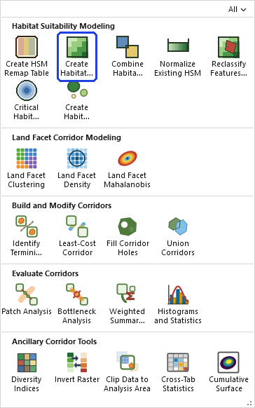
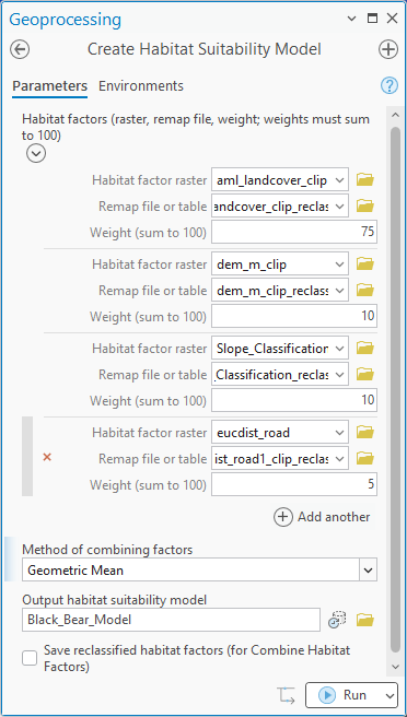
- Habitat factors. One block of three entries per factor: the raster, picked from the map or browsed to; its remap file or table, an ASCII file or a geodatabase table; and its weight. Add another appends a block, and the red × beside a block removes it. Order matters in one way only: the first factor sets the output grid coordinate system, extent and cell size, so choose your first layer accordingly.
- Method of combining factors. Geometric Mean or Additive Mean, as above.
- Output habitat suitability model. The name and location of the result. A name inside a geodatabase gives a geodatabase raster; a name in a folder gives a GeoTIFF.
- Save reclassified habitat factors. Unchecked, only
the model is written. Checked, the per-factor
_rrasters are written beside it for Combine Habitat Factors.
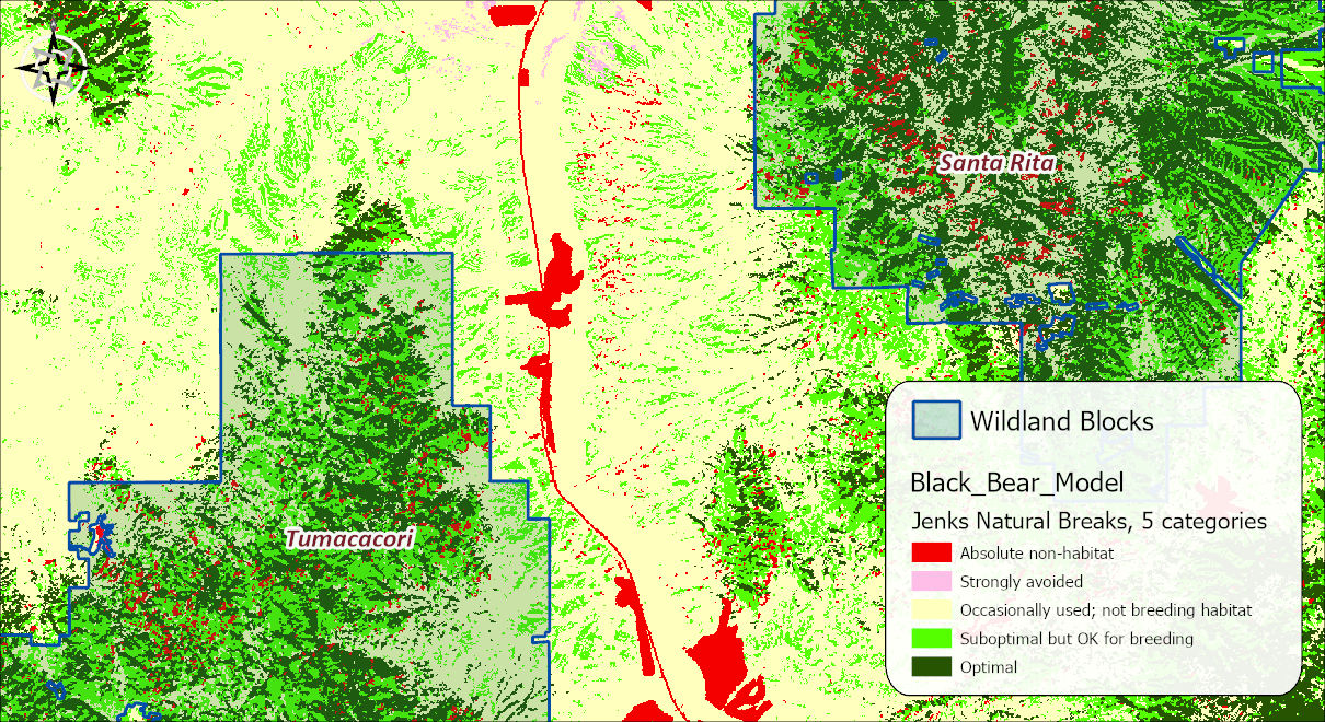
The five classes on the map deserve a word. The breaks come from Jenks natural breaks on the model's values, and the labels are the workshop book's anchors from absolute non-habitat to optimal. That is a reasonable draft, and only a draft: the method finds gaps in the distribution of scores and knows nothing about the species. If the expert says that anything below 30 is non-habitat, or that breeding habitat begins at 60, open the layer's symbology and move the breaks to those values.
The tool holds all of its raster data in memory at once, so the memory it needs grows with the number of cells. On most rasters that is no concern. On a very large one the tool may need more memory than your computer has free, and then one of two things happens: Windows starts using the disk as overflow memory and the tool slows to a crawl, or the tool stops with an out-of-memory error. There is no fixed limit; it depends on how much memory your computer has free. If your rasters are too large, clip them to the area you need first.
ModelBuilder
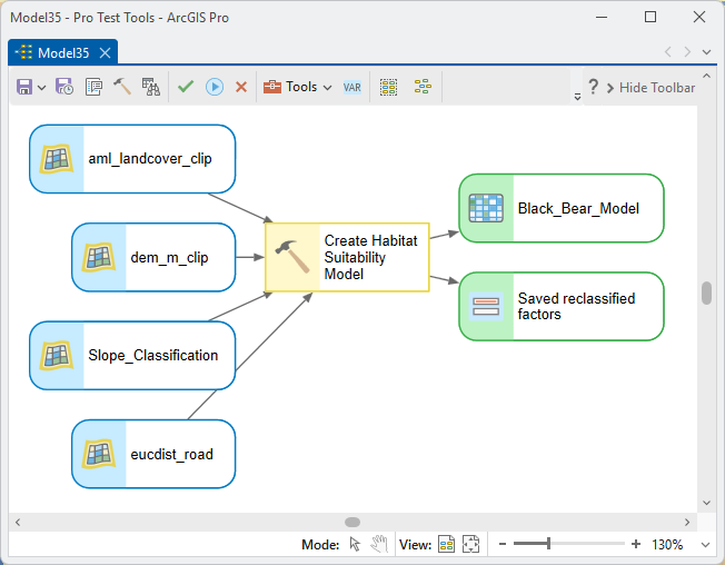
Parameters
| Label | Explanation | Data type |
|---|---|---|
| Habitat factorsRequired · factors | One row per factor: the raster, its remap file or table, and its weight. Any number of rows; weights must be positive and sum to exactly 100. The first row defines the output grid; other factors on a different grid are resampled onto it by nearest neighbour, with a message. | Value Table |
| Method of combining factorsRequired · method | Geometric Mean (the default and the workshop book's recommendation; a zero in any factor zeroes the cell) or Additive Mean (equivalent to Esri's Weighted Overlay; deficiencies average away). Both stay on 0–100. | String |
| Output habitat suitability modelRequired · out_raster | The 0–100 suitability raster, on the first factor's grid, symbolized on delivery and carrying statistics and provenance metadata. A folder path without an extension becomes a GeoTIFF. | Raster Dataset |
| Save reclassified habitat factorsOptional · save_reclassified | Checked: each factor's 0–100 reclassification is
also written beside the output with an _r
suffix, added to the map and listed in the messages, for
reuse in Combine Habitat Factors. Unchecked (default):
only the model is written. |
Boolean |
Python
import arcpy
arcpy.ImportToolbox(r"C:\path\to\JennessEnterprisesTools.pyt")  # your install path
arcpy.jenness.HabitatSuitabilityModel(
    factors="lndcvr_clip 'D:\\species\\blackbear_lndcvr.txt' 40;"
            "dem_clip 'D:\\species\\blackbear_elev_m.txt' 20;"
            "topo 'D:\\species\\blackbear_topo.txt' 20;"
            "dstroad 'D:\\species\\blackbear_dstroad.txt' 20",
    method="Weighted geometric mean",
    out_raster=r"D:\corr.gdb\blackbear_hsm")
Recommended citation
Credits and references
By Jeff Jenness, Jenness Enterprises (www.jennessent.com), ported from the CorridorDesigner tools by Jenness, Majka and Beier.
- Beier, P., D. Majka, and J. Jenness. 2007, revised 2026. Designing wildlife corridors with ArcGIS: ArcGIS Pro edition. Workshop book, revised by J. Jenness for the Corridor Designer Tools of the Wildlife and Forestry Tools add-in. Available at: CorridorDesigner_WorkshopBook_2026_ArcGISPro.pdf (5 MB)
- Beier, P., D. Majka, and J. Jenness. 2007. Designing wildlife corridors with ArcGIS. Workshop book, Northern Arizona University. Available at: corridordesign.org (archived copy at the Internet Archive)
Licensing information
Works at every ArcGIS Pro license level (Basic, Standard, Advanced). No extension licenses are required.
Related tools and pages
- About Corridor Design — the habitat-modeling theory: factors, scoring, and the fundamental assumption.
- Corridor Design Tutorial — this tool in the full workflow, with the black bear example.
- Create Habitat Patches — the next step in the chain.