

Cross-Tab Statistics
Summary
Builds a cross-tabulation (contingency) table — a
two-dimensional histogram showing how much of the landscape falls in
each joint range of two variables. Sources: two fields of one
table or feature class (weighted equally, by an attribute, or by
geodesic feature size); two polygon layers (intersection regions,
area-weighted); two rasters (paired cell values); or a polygon layer
against a raster, sampled per cell or per polygon with a zonal
statistic. The variables can be numeric or categorical: a
text field such as an ownership type or a land-cover name becomes
one class per distinct value, already labeled, and a raster takes
its class names from its layer's unique-value symbology or from a
name column in its attribute table — or is regrouped
outright by any text column of that table, so a table with a
Land Cover attribute field with 26 different land
cover classes and an NLCD attribute field with 10
NLCD classes can be grouped and tabulated by either
Land Cover or NLCD. Landfire EVT
(Existing Vegetation Type) rasters are a good example of this:
they often have many different classification systems available
in the attribute table.
Land cover by ownership comes out with every row and column
named, nothing to type, and a per-polygon majority
statistic gives the dominant class of each polygon when one
observation per polygon is the right unit. (Names joined to a raster with a map-level Add Join
live only in the layer and are not visible to the tool; use
Join Field to write them into the attribute table.)
Optionally restricts everything to an analysis polygon.
Class names and ranges can be edited live; the table shows counts,
sizes (hectares, acres, …) or percentages, and can be copied,
exported to a geodatabase / dBASE / CSV table, or placed on a layout
as editable graphics. A modernized port of the CorridorDesigner
Evaluation Tools' Cross-Tab Statistics; no Spatial Analyst needed.
In corridor evaluation
The two-variable cousin of Weighted Summary Statistics: where that tool summarizes one variable at a time, this window crosses two — land cover by ownership inside a linkage polygon, habitat suitability class by slope class, corridor coverage by parcel. Restricting everything to an analysis polygon makes it a natural evaluation instrument: the classic workshop example crossed a proposed linkage against a parcel map to show exactly who owns how many acres of it.
A tour of the window
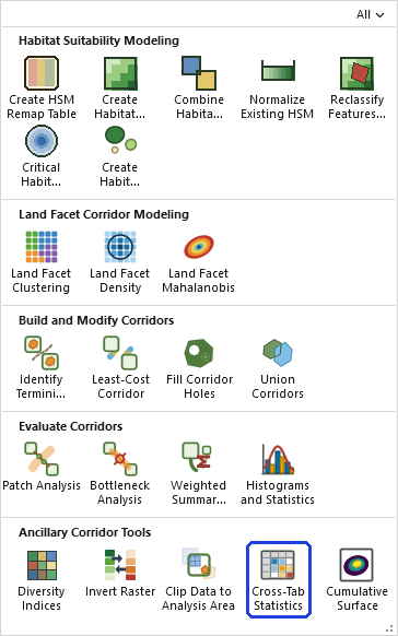
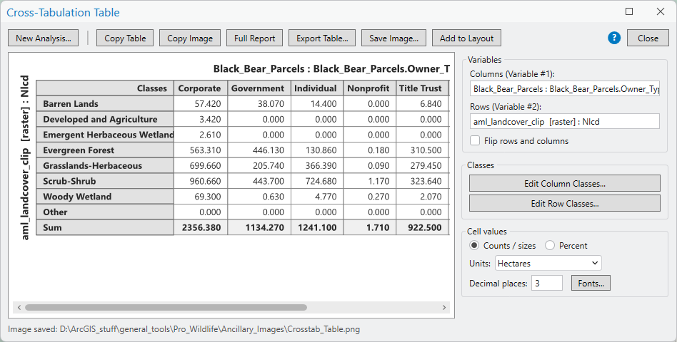
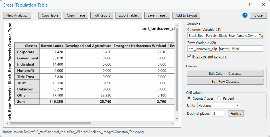
The example is the land-cover-by-ownership table from the Corridor Evaluation Tutorial: a parcel layer classed by owner type against a land-cover raster, inside a corridor polygon. The input dialog opens with the window; New Analysis... brings it back.
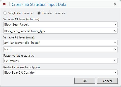
Nlcd here) regroups
the cells by it. Every control has hover help.A definition query is always honored, on a layer or table that supplies a variable and on the analysis polygon layer alike: the window works with the records each layer shows. When both variables come from one table or feature class, Selected records only narrows those records to the current selection.
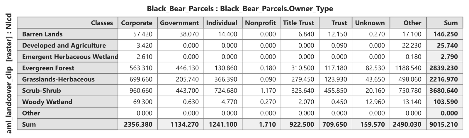
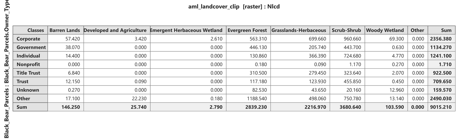
What the table shows, in this case, is where the corridor's 9,015 hectares sit. Three land-cover groups account for almost all of it: scrub-shrub, evergreen forest and grassland, in that order. Developed and agricultural land comes to 26 hectares, under a third of one percent, which is the most reassuring number in the table and one that the parcel layer alone could not have given. Down the columns, the owner types differ in kind rather than in amount: individually owned ground is mostly scrub, the small lots at the low western end; government ground splits evenly between forest and scrub; and the family trusts hold the scrubbiest ground of all. The two Other lines the tool always includes are worth a look too. The Other row is zero, because every raster cell belongs to a land-cover group. The Other column is not: 2,490 hectares, 28% of the corridor, which is corridor ground inside no parcel at all, public land outside the county's parcel fabric and road rights-of-way, and it is the most heavily forested column in the table. Anyone planning a linkage here would want to know that the best forest in the corridor is not on anybody's tax roll. The tutorial reads the table line by line.
Flipping rows and columns
Which variable runs across and which runs down is a presentation choice, not an analysis choice, so the window lets you change it after the fact: the Flip rows and columns checkbox transposes the table without re-reading anything. A table with few columns and many rows reads well on a portrait page; flipped, the same numbers fit a wide layout. Every export — image, text, table, layout graphics — follows the current orientation.
Cells or polygons: the raster variable statistic
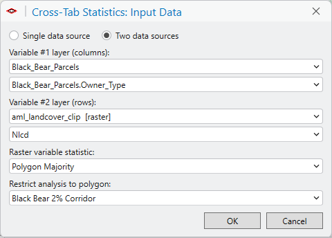
With a polygon layer against a raster, the Raster variable statistic decides what one observation is. It changes the numbers, not just their precision, so it is worth seeing the same data both ways.
Cell Values takes one observation per raster cell, each cell paired with whatever polygon it falls in and weighted by its own area. That is the table shown above: 9,015 hectares of corridor, every cell counted, including the 2,490 hectares in the Other column that fall inside no parcel at all.
Polygon Majority takes one observation per polygon: the class covering the most of that polygon's cells, weighted by the polygon's own area. Run the same inputs that way and the table changes character.
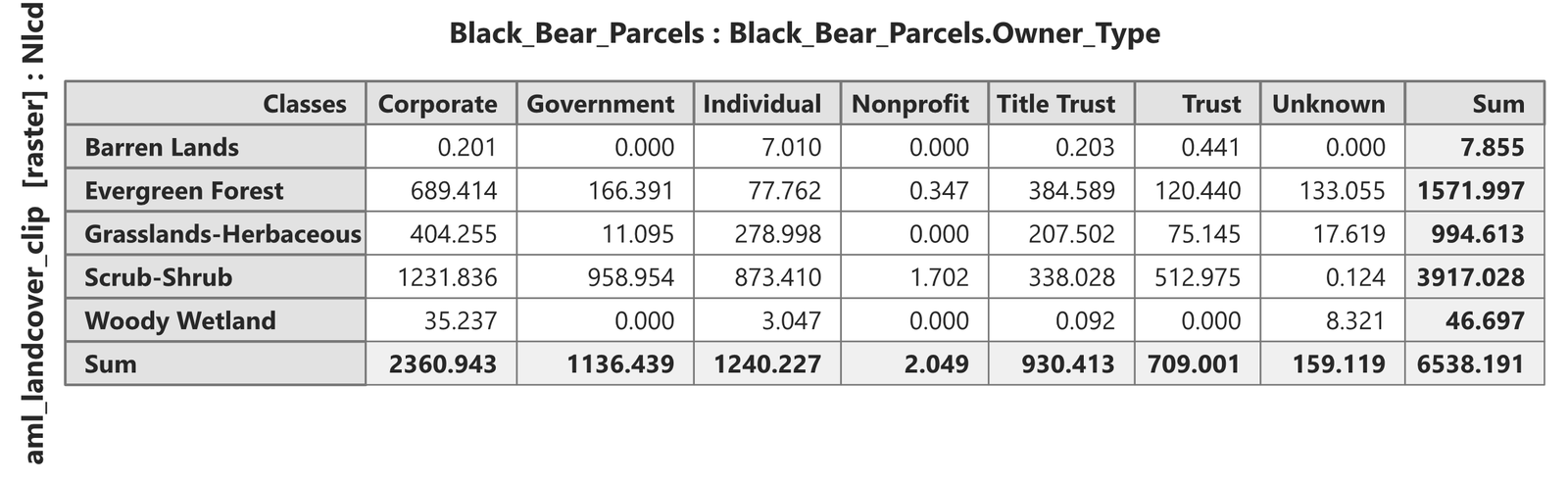
Three things differ, and each is a consequence of the unit of observation. First, there is no Other column and the total is 6,538 hectares, not 9,015: the observations are parcels, so ground in no parcel is simply not observed. Second, minority classes vanish into their neighbors — the developed and emergent-wetland rows are gone and barren lands drop from 146 hectares to 8, because a parcel that is mostly scrub with a strip of wash counts entirely as scrub. That is the point of the majority: it answers “what kind of parcel is this?”, not “what is on each acre?”. Third, even the column totals differ slightly — corporate ground is 2,356 hectares by cells and 2,361 by parcels — and that is a matter of measurement. Cell Values measures a parcel as the number of 30-meter cells whose centers fall inside it, times a cell's area; Polygon Majority measures it as its exact geodesic area. Over 1,564 parcels, some smaller than a single cell, the two disagree by about two tenths of one percent. When the totals must reconcile with a parcel table, use the polygon statistics; when the question is about the ground itself, use the cells.
The remaining polygon statistics — mean, minimum, maximum, range, standard deviation, sum — also take one observation per polygon, but summarize its cells as a number, which only makes sense for a continuous raster: elevation, suitability, distance. A mean of land-cover codes means nothing, which is why they are withheld whenever a raster is grouped by an attribute column. Against a continuous raster they come into their own:
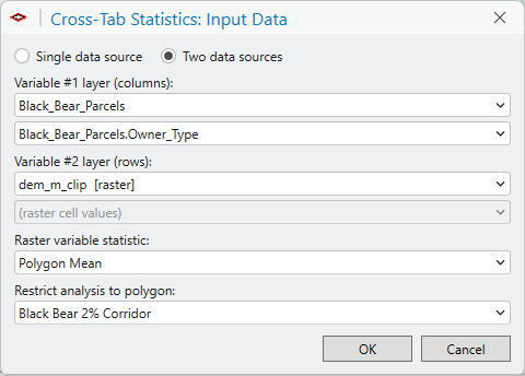
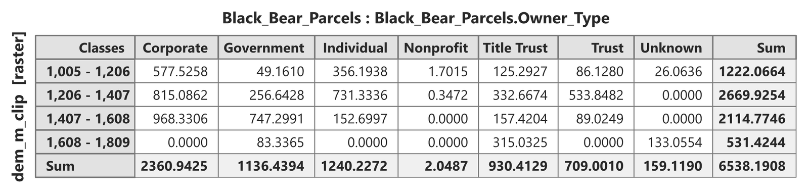
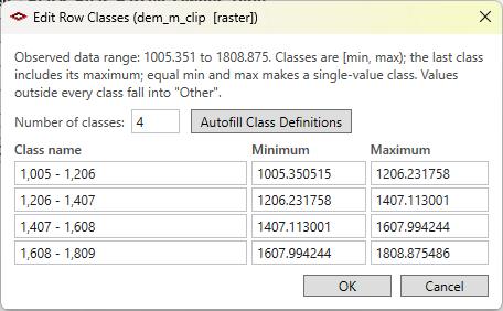
For a continuous variable the classes are yours to define. Edit Row Classes... (or Column Classes) opens the class editor: set the number of classes and Autofill for equal intervals over the observed range, or type any minimum, maximum and name per class — 1,000 to 1,500 meters and 1,500 to 2,000, say, or classes that match a published elevation zonation. Classes are half-open (minimum ≤ value < maximum), the last class includes its maximum, equal minimum and maximum make a single-value class, and anything outside every class lands in Other. The table rebuilds as soon as you click OK; nothing is re-read.
Sizes or percentages
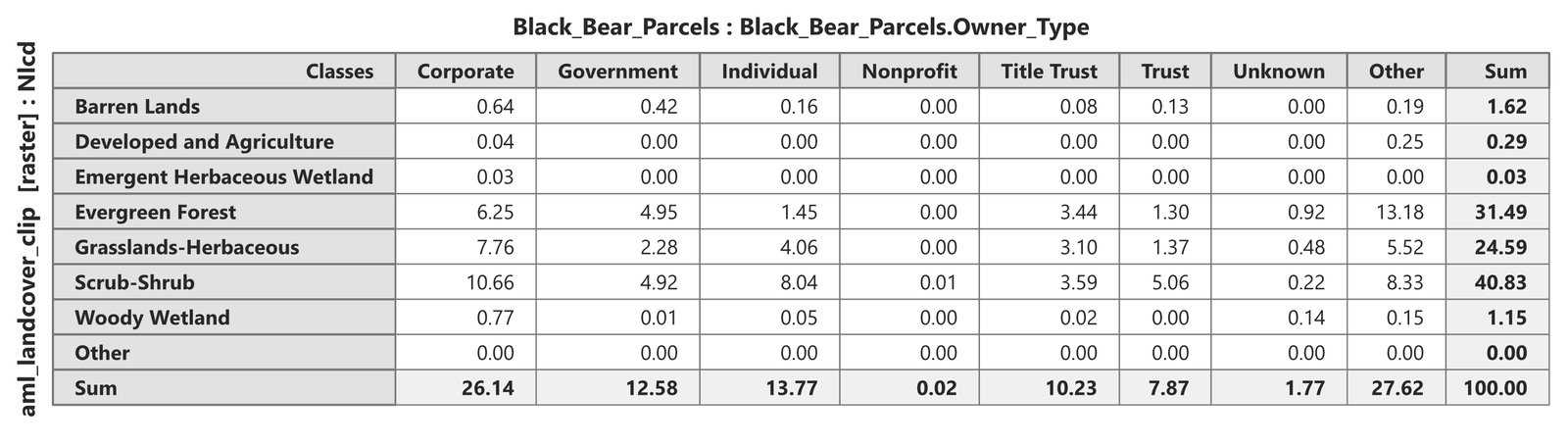
The Cell values group in the side panel switches the whole table between sizes and proportions. Counts / sizes shows each cell in the chosen unit — hectares, acres, square kilometers, square miles, or the native cells or record count. Percent shows each cell as its percentage of the grand total, so the table sums to 100; the row and column sums then read directly as each class's share of the whole. The Decimal places box applies to either view, and matters more for percentages, where a small class can disappear into 0.0 at one place and reappear at three.
Recommended citation
Credits and references
By Jeff Jenness, Jenness Enterprises (www.jennessent.com), modernizing the CorridorDesigner Evaluation Tools' Cross-Tab Statistics (Jenness, Majka and Beier).
- Beier, P., D. Majka, and J. Jenness. 2007, revised 2026. Designing wildlife corridors with ArcGIS: ArcGIS Pro edition. Workshop book, revised by J. Jenness for the Corridor Designer Tools of the Wildlife and Forestry Tools add-in. Available at: CorridorDesigner_WorkshopBook_2026_ArcGISPro.pdf (5 MB)
- Jenness, J., D. Majka, and P. Beier. 2014. CorridorDesigner Evaluation Tools. Available at: corridordesign.org (archived copy at the Internet Archive)
Licensing information
Works at every ArcGIS Pro license level (Basic, Standard, Advanced). No extension licenses are required.
Related pages
- Weighted Summary Statistics — the numbers behind one variable at a time, weighted by area or length, where this window crosses two.
- Histograms and Statistics — the distributions behind the same variables.
- Classification Accuracy (Kappa) — when the two categorical variables are a prediction and a reference, the contingency table becomes an error matrix with a full inferential report.
- About Kappa and classification accuracy analysis