Corridor Designer Tools · Evaluate Corridors ·
interactive window + geoprocessing tool · by Jeff Jenness
Works at every ArcGIS Pro license level
Summary
Finds the route through a corridor polygon between two
wildland blocks that maximizes the minimum corridor width
encountered — the route with the widest bottleneck,
chosen over every strand and branch of the corridor at once
— and measures the corridor width at regular stations
along it. A narrow spot is a bottleneck, and for species
sensitive to edges or development a severe bottleneck can make
a corridor useless; this analysis shows exactly where the
corridor narrows, by how much, and for how long. Compare the
narrowest point against what your species tolerates —
and where a pinch is not constrained by hard edges,
that is where widening the corridor buys the most. A
modernized port of the CorridorDesigner Evaluation Tools'
Bottleneck Analysis; no Spatial Analyst needed.
The corridor's medial axis — its skeleton,
where every point is the center of a circle touching the
boundary on two or more sides — is computed exactly in
vector from a Voronoi construction, with the local corridor
half-width known at every point. The route through that
skeleton maximizing the minimum width is found over all
strands and branches simultaneously, so the answer is exact
— no raster approximation, widths and lengths in
meters. An optional width threshold classifies the route into
above- and below-threshold stretches.
Window and geoprocessing tool
The interactive window is where the exploration
happens: run the analysis, then drag the width threshold and
watch the statistics, the width-profile graph, and the
highlighted sub-threshold stretches update live; place the
graph on a layout when it tells the story. The
geoprocessing tool runs the same underlying analysis as
a scripting and batch surface — ModelBuilder chains, many
corridors in a loop — and produces the same three
outputs: the route polyline, optional station points with
widths, and optional above/below-threshold segments, each
carrying the analysis record. What the geoprocessing,
ModelBuilder and Python scripting options do not include is
the window's interactivity: no live graph to drag a threshold
on, and no way to place a graphic or a statistics text element
on a layout — those belong to the window alone. Run it
once per threshold you care about, and use the window when you
want to explore.
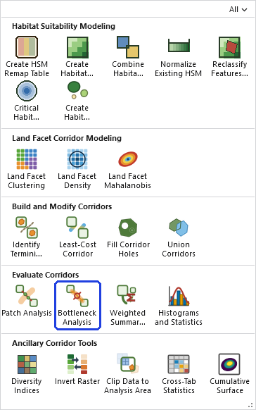
Where to find it: Bottleneck Analysis is in the Evaluate Corridors
row of the Corridor Designer Tools gallery, in the Corridor Designer Tools group of the
Wildlife and Forestry tab.
Corridor and blocks
The corridor polygon must be a single polygon: the
tool finds one best route, and a corridor made of several
disconnected strands (common straight out of Least-Cost
Corridor, whose slices can sprout branches) has no single
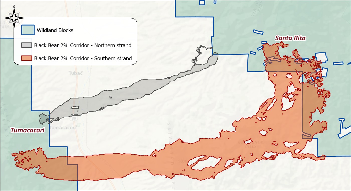
answer. Here that means picking one strand out of the black
bear 2% corridor — the wider one running south through
Tumacacori — rather than handing the tool every strand at
once.
The 2% black bear corridor is two disconnected
strands: a narrow northern one in gray and the broad southern
one in orange. The southern strand is the one handed to the
tool.
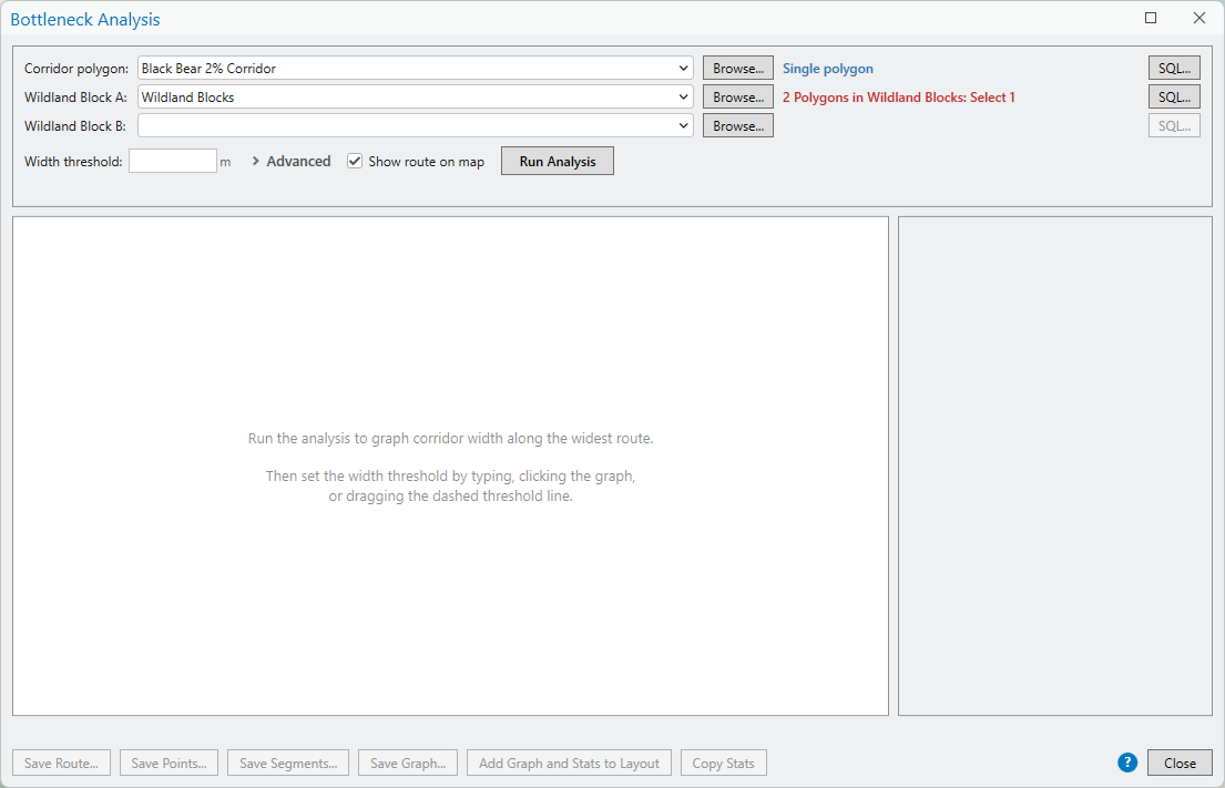
The status text beside each Browse button confirms what
the tool sees: Single polygon
in blue when a field is ready to run, or a count in red when it
is not.
The two wildland blocks are usually two features in the
same feature class, which is exactly the case here: both
Wildland Block A and Wildland Block B point at the same
Wildland Blocks layer. The tool notices there is
more than one feature and asks you to narrow each field down to
one, with a live count: 2 Polygons
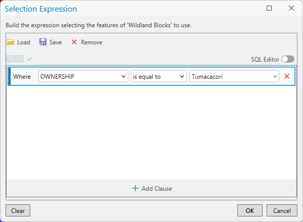
in Wildland Blocks: Select 1. The SQL... button
beside each field opens the same query builder used throughout
the add-in, so you can pick the block by an attribute rather
than by selecting it on the map first.
Corridor polygon is ready (a single polygon);
Wildland Block A points at a two-feature layer and needs its
own SQL expression before the tool can run.The SQL query builder, narrowing Wildland Block A
to the Tumacacori feature. Block B gets the same treatment
with OWNERSHIP = 'Santa Rita'.
With both blocks resolved to one feature each and a width
threshold typed in, click Run Analysis.
Reading the result
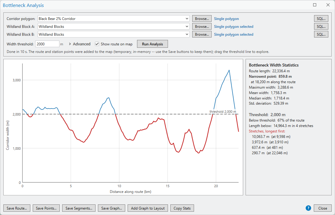
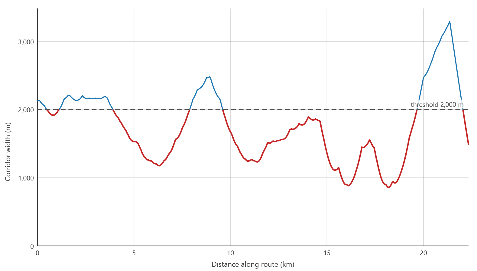
The graph plots corridor width against distance along the
route; the statistics panel on the right reports the route
length, the narrowest point and where it falls, and the mean,
median and standard deviation of width along the whole route.
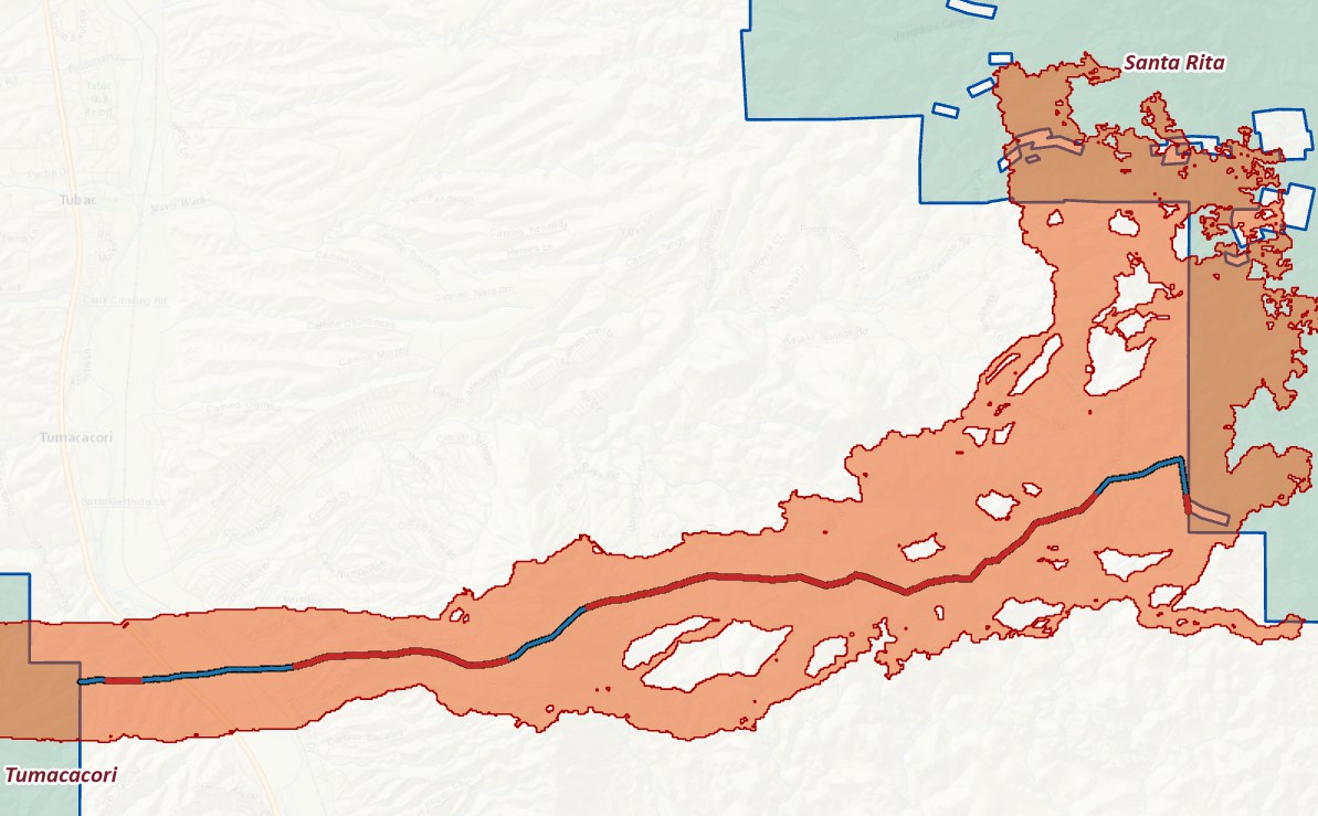
With a threshold set, both the graph and the statistics split
at that value: the graph colors the profile blue above the
threshold and red below it, and the map does the same to the
route line, so a glance at either one shows where the corridor
is comfortable and where it pinches.
The window at a 2,000 m threshold: 67% of
the route falls below it, across four stretches, the
longest running 10,063.7 m.The same result on the map, colored to
match.
Adjusting the threshold
Change the threshold by typing a new value, clicking a point
on the graph, or dragging the dashed threshold line itself up
or down — no need to rerun the analysis, since the width
profile was already computed once and every number and color
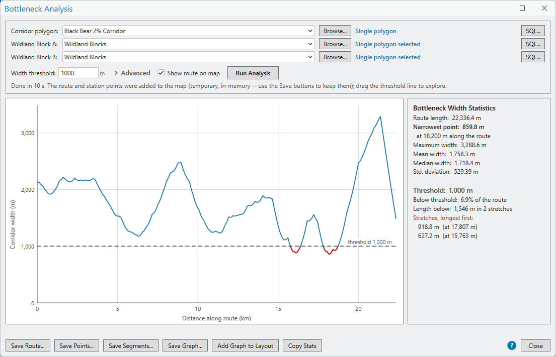
below the line simply reflects wherever it now sits. Suppose,
after seeing the 2,000 m picture, you decide that 2,000
was too cautious and the corridor really only becomes a problem
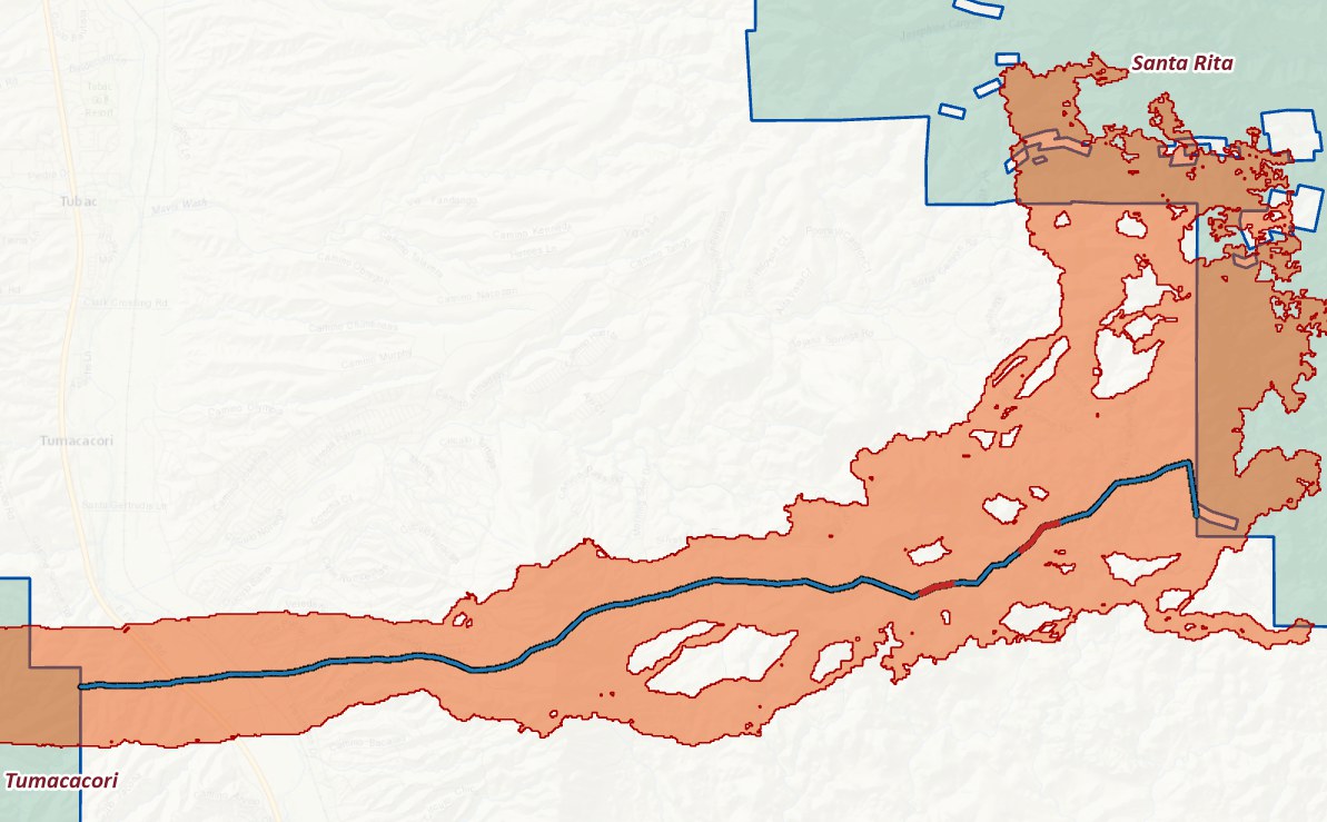
below 1,000 m. Move the threshold down and the story
changes completely: only 6.9% of the route now falls below it,
in two short stretches instead of four long ones.
The threshold moved to 1,000 m: the same
route, but now only 6.9% of it counts as a
bottleneck.The map follows instantly: almost the entire
route is comfortable at this looser threshold.
Advanced options
Three controls, tucked under the Advanced expander,
tune the analysis without changing what it measures:
Stations — how many points along the route
the width is sampled at (default 1,000). More stations trace
the profile more finely; the default is enough to catch a
bottleneck a few meters wide on a corridor several kilometers
long.
Boundary sampling (m) — the spacing used
when building the Voronoi skeleton from the corridor
boundary. Left blank, the tool picks a spacing scaled to the
corridor's own size (the extent diagonal divided by 2,000).
A finer spacing traces a more detailed boundary at the cost
of a slower run; it rarely needs to be set by hand.
Simplify tolerance (m) — simplifies the
corridor boundary before analysis. Blank means automatic, 0
means no simplification at all. A boundary with a great many
vertices (a corridor sliced from a fine-resolution raster,
say) can be simplified without changing the medial-axis
answer in any way that matters, and the run finishes faster
for it — the same trade the Patch
Analysis tool offers for the same reason.
The Show route on map checkbox controls only whether
the route and its colored stretches draw as a temporary overlay
while you work; it has no effect on the analysis or on what you
can save afterward.
Getting results out
Six buttons along the bottom of the window cover every way
to keep what the analysis produced:
Save Route..., Save Points..., Save Segments...
write the route polyline, the width-measurement stations, or
the above/below-threshold pieces of the centerline to a real
feature class — the map view shows everything
in-memory until you do. Save Segments is the one
behind the colored route in the layout figure below.
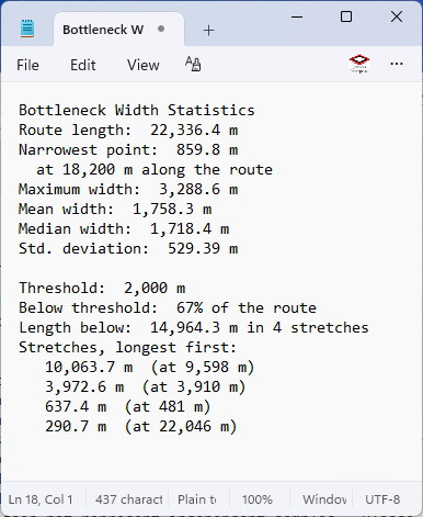
Copy Stats puts the statistics panel on the
clipboard as plain text, ready to paste into a report or an
email. You can also select text directly out of the panel
with the mouse and copy just the lines you need, the way you
would from any document.
Copy Stats, pasted straight into a text
editor.
Save Graph..., exported as a PNG at the 2,000 m
threshold.Save Graph... exports the width-profile graph as a
PNG image or an SVG vector file, for a report or presentation
that is not built as an ArcGIS Pro layout.
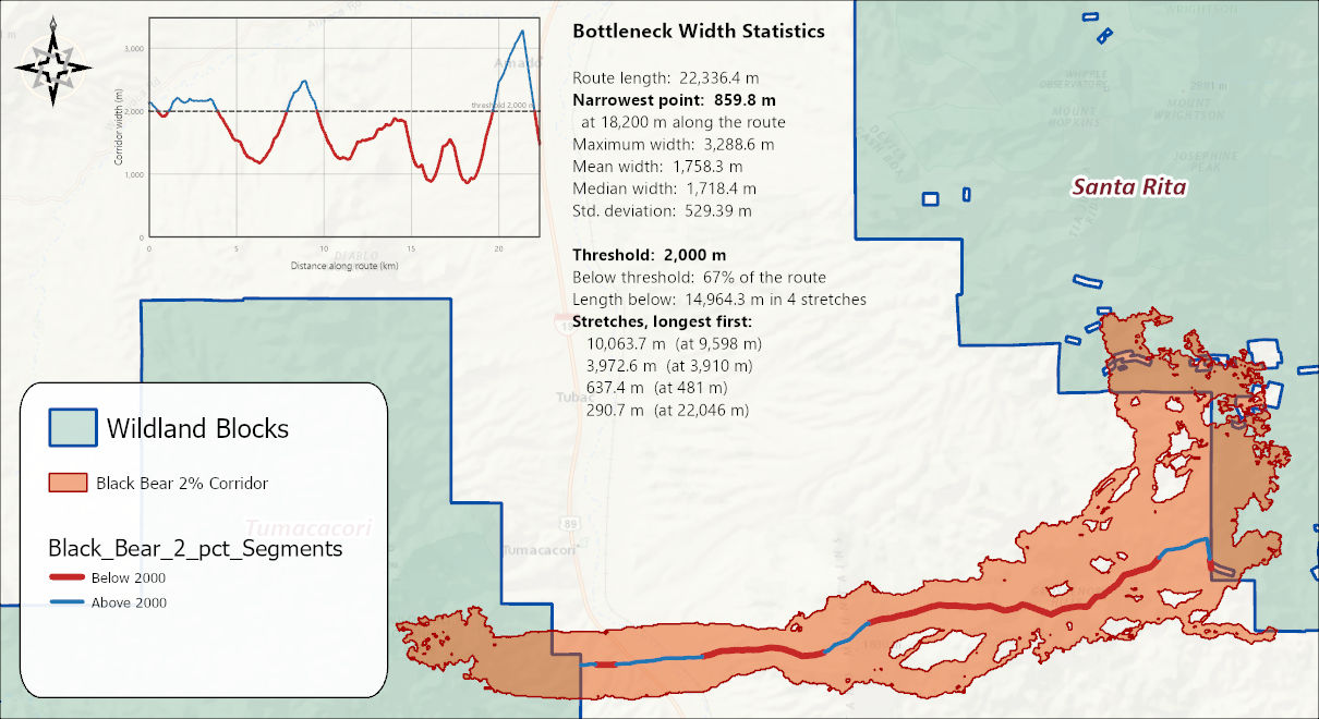
Add Graph and Stats to Layout places the graph
and the statistics on a layout together, as native,
individually editable graphic and text elements — not a
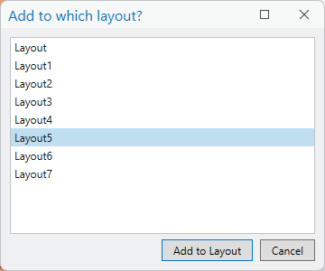
picture. If a layout is the active view, it goes there
directly; otherwise you are asked which of the project's
layouts to use, or, if the project has none yet, pointed to
Insert ▸ New Layout.
Add Graph and Stats to Layout: the graph and its
statistics as native layout elements, beside the corridor with
the saved threshold segments symbolized on the map.If the active view is a map rather than a layout
when you click Add Graph and Stats to Layout, the tool asks
which layout to use.
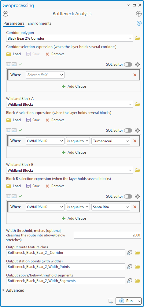
The geoprocessing tool, and ModelBuilder
The geoprocessing tool takes the same inputs as the window
— a corridor polygon, the two wildland blocks (with the
same per-field SQL expressions when a layer holds more than
one feature, as in the black bear example above), and an
optional width threshold — and writes the route, the
station points, and the above/below-threshold segments
directly to named output feature classes, no window required.
The advantage of this version of the tool is that it can be run
from a Python script or chained into a string of tools in
ModelBuilder, so one model can evaluate every corridor in a
project the same way. The downside is that you cannot easily
explore the consequences of different thresholds, since each
threshold is a separate run rather than a drag on a live graph,
and you cannot create graphics for your layouts or reports; both
of those belong to the window.
The same black bear inputs as the window,
including the same two SQL expressions, with three named
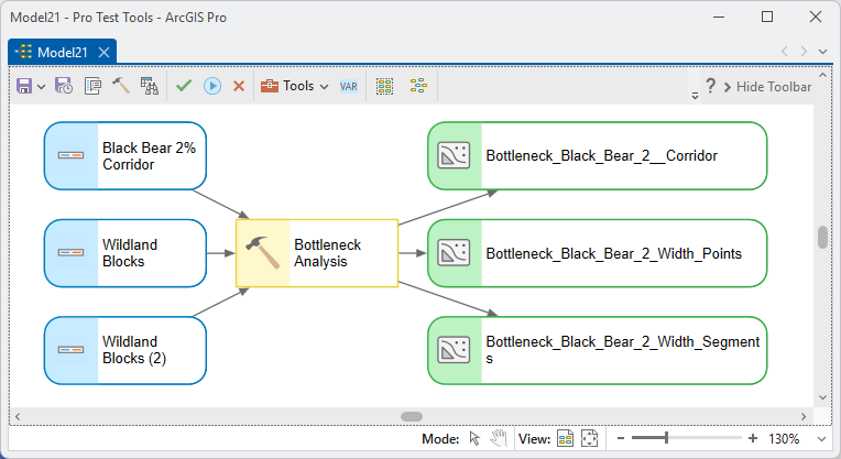
outputs.In ModelBuilder: the corridor and the two block
selections in, the route, width points and threshold
segments out.
Parameters (geoprocessing tool)
Label
Explanation
Data type
Corridor polygonRequired · corridor
The corridor to profile. An active selection is honored.
The dialog lists one more parameter, Profile JSON
path. It is used by the Bottleneck Analysis window to
receive the width profile and should be left blank.
Jenness, J., D. Majka and P. Beier. 2026.
Bottleneck Analysis. Wildlife and Forestry Tools add-in
for ArcGIS Pro, v. 1.99 (September 2026). Jenness
Enterprises. Available at:
https://github.com/JeffJenness/Wildlife_Tools.
Credits and references
By Jeff Jenness, Jenness Enterprises
(www.jennessent.com),
ported from the CorridorDesigner Evaluation Tools by Jenness,
Majka and Beier.
Beier, P., D. Majka, and J. Jenness. 2007, revised 2026.
Designing wildlife corridors with ArcGIS: ArcGIS Pro
edition. Workshop book, revised by J. Jenness for the
Corridor Designer Tools of the Wildlife and Forestry Tools add-in.
Available at:
CorridorDesigner_WorkshopBook_2026_ArcGISPro.pdf (5 MB)
Jenness, J., D. Majka, and P. Beier. 2014.
CorridorDesigner Evaluation Tools. Available at:
corridordesign.org (archived copy at the Internet Archive)
Licensing information
Works at every ArcGIS Pro license level (Basic, Standard,
Advanced). No extension licenses are required.