Land Facet Tutorial

Corridor Designer Tools · tutorial · by Jeff Jenness

This tutorial walks a complete land facet corridor analysis with the ArcGIS Pro tools — the workflow from the original Land Facet Corridor Designer manual, considerably streamlined. The original toolkit shuttled data out to R for the clustering statistics and back; the Pro tools run the entire chain inside ArcGIS, and each step stamps a provenance record that the next step validates, so a mismatched input is caught instead of silently accepted. The concepts — and the reasons this approach shrugs off climate change — are on the About Land Facet Corridors page.

The shape of the analysis Define land facets from enduring terrain → build one cost surface per facet (plus one for facet diversity) → run a least-cost corridor on each → union the strands into the linkage design. Expect roughly 8–16 facets and a dozen corridor strands.

Step 1: A first-pass classification

Start from a raster that carves the landscape into broad classes, each of which will be subdivided into land facets. The classic choice is topographic position, and the tutorial uses the same tool and classification the Corridor Design Tutorial used for its habitat model: Slope Position Classification on the tutorial DEM, with the TPI and slope computed on the fly, a circular neighborhood of 10 cells (300 m on this 30 m grid), raw TPI in elevation units, geodesic slope in degrees, and the Corridor Designer 4-Class Topographic Position system. That system reads canyon bottoms as cells at least 12 m below their neighborhood mean, ridgetops as cells at least 12 m above it, and splits everything between at a 6° slope into flat-gentle and steep slopes. The original land facet work used three positions, canyon, slope and ridge; four works just as well, and it lets the clustering treat gentle and steep ground separately from the start. If neither the Corridor Designer system nor the other bundled ones (Weiss's six classes, Dickson and Beier's four, the Land Facet three) suits your landscape, the Classification System Builder lets you define your own: the thresholds, the class names and the colors, saved under a name that then appears in the tool's list. A soil-type or landform raster works equally well if you have a good one — and if you prefer to classify the whole landscape in one pass, a constant raster serves as the single “class” containing everything.
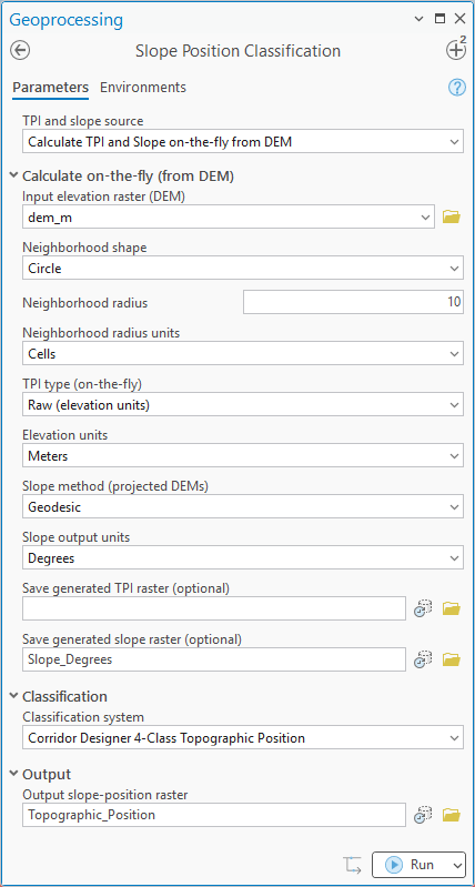
The Slope Position Classification geoprocessing pane: TPI and slope calculated on the fly from dem_m, circle neighborhood, radius 10 cells, raw TPI in elevation units, meters, the generated slope raster saved as Slope_Degrees, the Corridor Designer 4-Class Topographic Position system, output Topographic_Position
Slope Position Classification set up for the tutorial: TPI and slope from the DEM on the fly, a 10-cell circular neighborhood, raw TPI, and the Corridor Designer 4-class system. The generated slope raster is saved as Slope_Degrees, because it will be wanted again in Step 2.
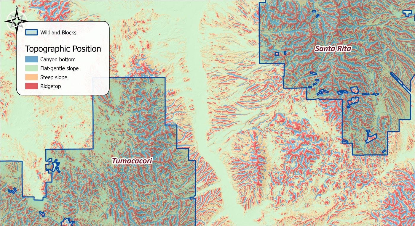
The topographic position raster over a hillshade: canyon bottoms in blue, flat-gentle slopes in pale green, steep slopes in tan and ridgetops in red, with the Tumacacori and Santa Rita wildland blocks outlined in dark blue
The four topographic positions with the wildland blocks outlined. Only the cells inside the blocks will be used to define the facets in Step 2; the classification covers the whole landscape so that Step 3 can score every cell between the blocks against them.

Step 2: Cluster each class into land facets

This is the step that once meant exporting tables, running a package of R functions, and importing the results back. Land Facet Clustering now does the whole thing in one window: it screens multivariate outliers, runs fuzzy c-means clustering across candidate cluster counts, applies the confusion screen to drop ambiguous cells, and writes one combined raster of uniquely numbered land facets. The facets are defined from the cells inside the wildland blocks only, since they should represent what the linkage connects. The window walks four pages, and the important thing to know before starting is that pages 2 and 3 are done once per class: with four topographic positions, that is four outlier screens and four clustering runs before the facet raster can be written.

The continuous variables

The tutorial follows the original work and clusters on three variables: elevation (the DEM itself), slope in degrees (the Slope_Degrees raster saved in Step 1), and annual solar insolation, computed from the DEM with the Spatial Analyst tool Area Solar Radiation for a whole year at a 14-day interval, in watt-hours per square meter. The original used insolation only for the slope classes, on the reasoning that canyon bottoms and ridgetops have no consistent aspect; the tutorial simply gives it to every class and lets the clustering decide how much it matters. Soil variables would join here wherever a decent soil map exists.
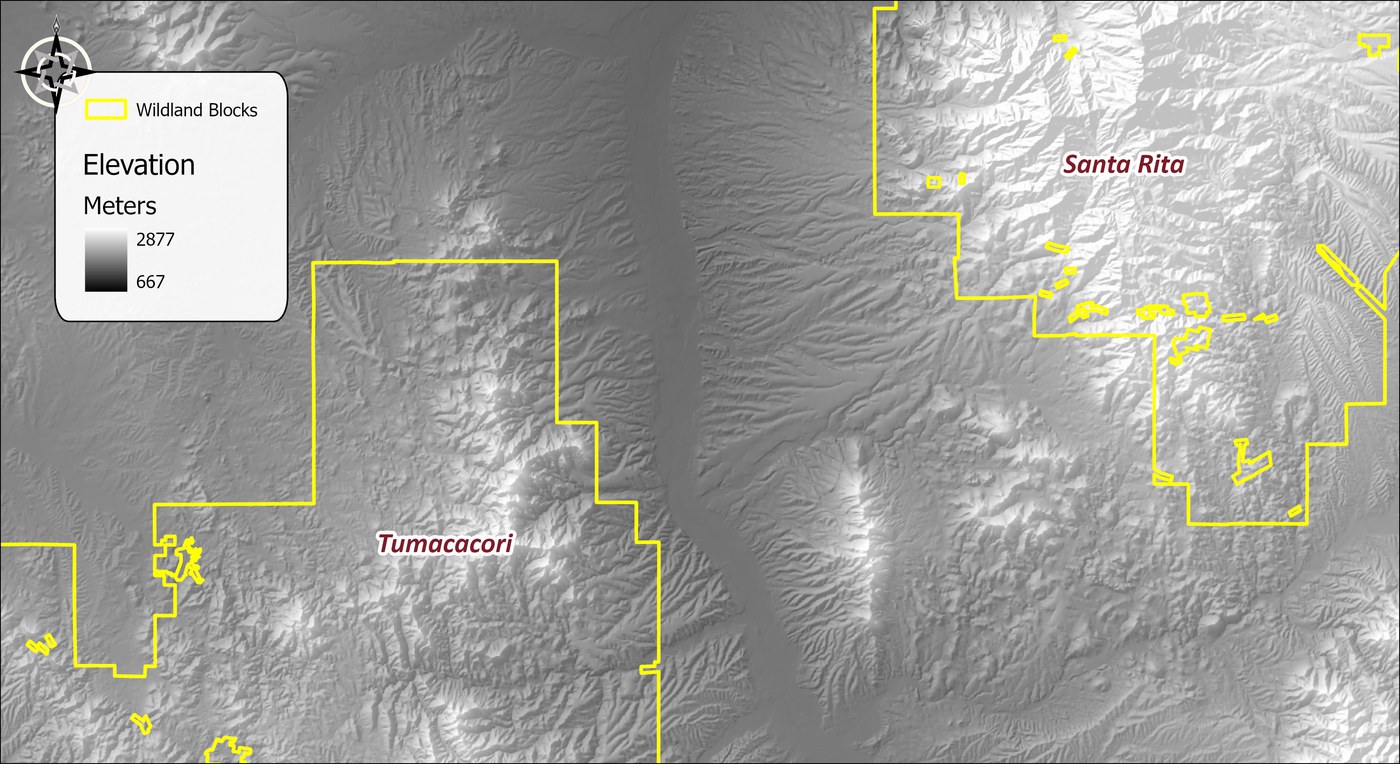
Elevation over the study area as a gray ramp from 667 to 2,877 meters, with the Tumacacori and Santa Rita wildland blocks outlined in yellow
Elevation, 667 to 2,877 m.
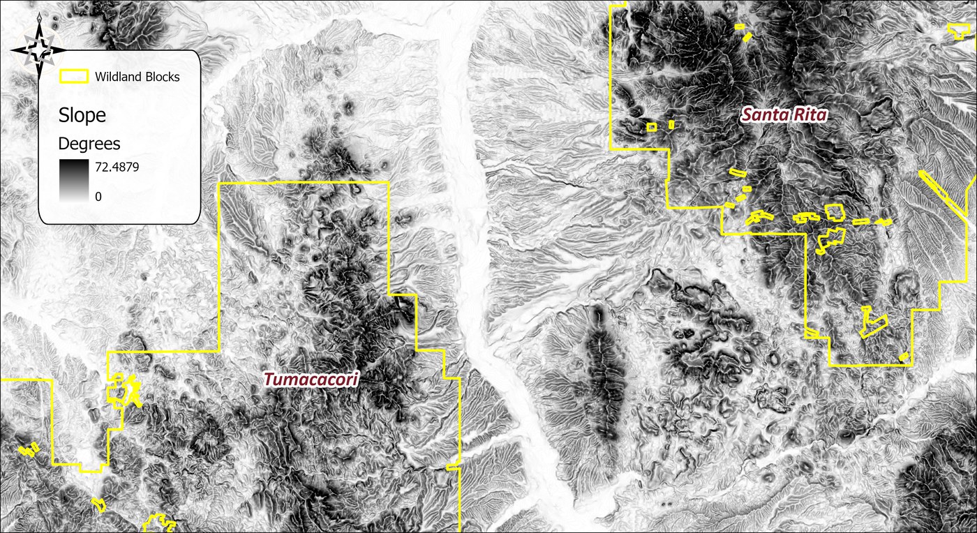
Slope in degrees over the study area, white on the flats to black on the steepest ground, with the wildland blocks outlined in yellow
Slope in degrees, from the Slope_Degrees raster saved in Step 1.
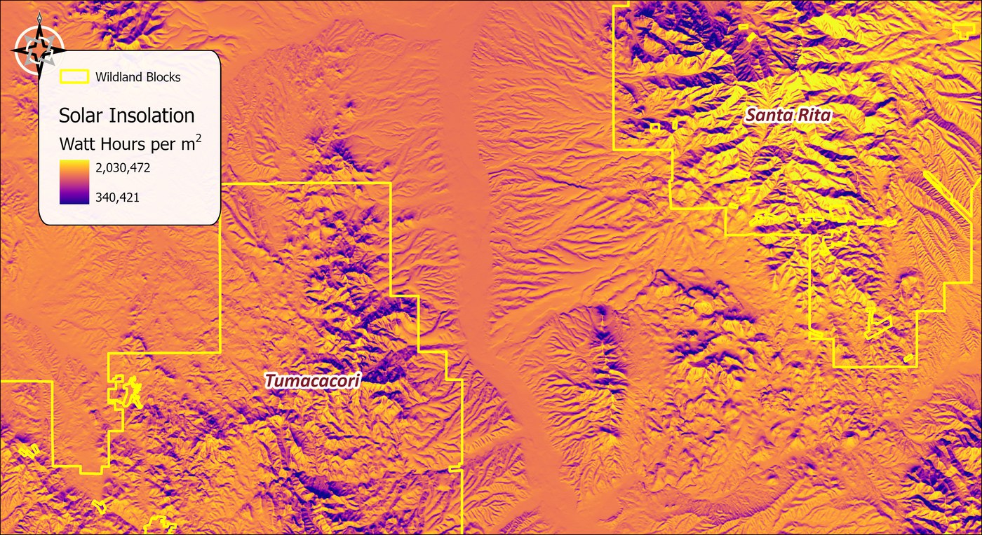
Annual solar insolation over the study area in watt-hours per square meter, from 340,421 in deep purple on shaded north-facing slopes to 2,030,472 in yellow on open south-facing ground, with the wildland blocks outlined in yellow
Annual solar insolation, 340,000 to 2,030,000 Wh/m²: purple on the shaded north-facing slopes, yellow on the sunny south-facing ones. This is the variable that separates warm from cool ground of the same elevation and steepness.

Page 1: Setup

Pick the categorical raster (Topographic Position), the wildland blocks as the clip polygon, and the three variable rasters (hold Control to select several), then click Read inputs. Nothing happens until you do: the window reads the rasters, finds the classes and counts the complete-case cells, here just over two million cells in four classes. The Export tables for R... button next to it writes the original Export-for-R tables from the data just read, for anyone who still prefers to run the fuzzy clustering in R; it is no longer necessary, and this tutorial does everything in Pro. One setting matters more than it looks: set Name classes by to the raster's Class_Name field, so that every report and legend from here on says “Ridgetop, cluster 2” rather than “Class 4, cluster 2”.
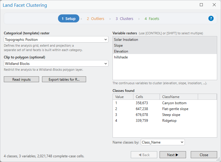
Land Facet Clustering, page 1 Setup: categorical raster Topographic Position, clip to polygon Wildland Blocks, Read inputs and Export tables for R buttons, variable rasters Solar Insolation, Slope and Elevation selected, classes found 1 Canyon bottom 358,673 cells, 2 Flat-gentle slope 647,238, 3 Steep slope 676,078, 4 Ridgetop 339,759, Name classes by set to Class_Name, status 4 classes, 3 variables, 2,021,748 complete-case cells
Setup after Read inputs: four classes inside the blocks, three variables, about two million complete cells. Name classes by has been switched from the raw value to the Class_Name field.

Page 2: Outliers

Cells with rare combinations of the variables, an unusually high, flat, sunny canyon bottom, say, would stretch the clusters across empty attribute space, so the method removes them first. The page draws a sample of each class, flags the least-dense fraction of it as outliers (10% by default; drag the slider or type a percentage), and shows them in red on a scatter plot of any two variables. Outliers are set aside from the clustering and left NoData in the facet raster. Choose each class in the Category list in turn and click Detect outliers for it; the list shows a check mark against each class that is set, and all four must be before the clustering page will work on them. The tool page shows how to change the plot axes to look at the sample from another pair of variables.
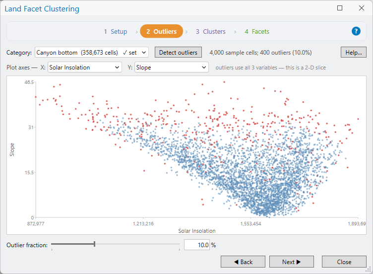
Land Facet Clustering, page 2 Outliers, for Canyon bottom: 4,000 sample cells, 400 outliers at 10 percent, a scatter plot of slope against solar insolation with the outliers in red around the sparse edges of the cloud, outlier fraction 10 percent
Canyon bottom: a 4,000-cell sample plotted as slope against insolation, with the 10% least-dense cells flagged in red. Repeat for each class in the Category list.

Page 3: Clusters

The same routine again: choose a class, click Run clustering, repeat for all four. For each class the window runs fuzzy c-means for every candidate cluster count from 2 to 7, twelve restarts each, and plots eight cluster-validity indices against the number of clusters. The restarts matter because c-means begins from randomly placed cluster centers and settles into whichever grouping is nearest that start, which is not always the best one; running it twelve times from twelve different starts and keeping the best result makes the answer repeatable rather than an accident of the first draw. More restarts cost time and rarely change the outcome; fewer risk a poor fit for one cluster count that throws the charts off. A consensus of the six clearest indices picks the suggested number, marked by the dashed line on every chart. The How to read these charts... button explains each index and which direction is better.
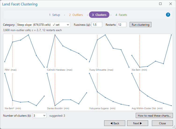
Land Facet Clustering, page 3 Clusters, for Steep slope: fuzziness 1.5, 12 restarts, eight small charts of validity indices against the number of clusters with a dashed line at 3, number of clusters 3, suggested 3
Steep slope: 3,600 non-outlier sample cells, cluster counts 2 to 7 tried, and the indices agree on three clusters.

The suggestion is a starting point, not a verdict. The Number of clusters box is yours to change, and the dashed line moves with it so you can see how your choice sits against each index. Ridgetops, for instance, came back with a suggestion of six, more ridge facets than this landscape seems to need; four is a defensible reading of the same charts, and simpler facet maps are easier to interpret and to defend later.
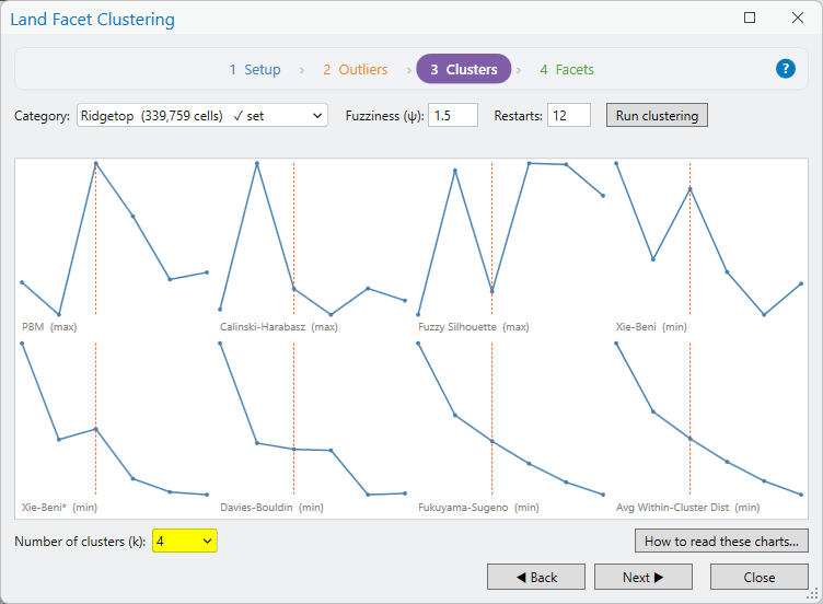
Land Facet Clustering, page 3 Clusters, for Ridgetop: the eight validity charts with the dashed line moved to 4 after the number of clusters was changed from the suggested value to 4
Ridgetop with the cluster count changed by hand to four; the dashed line moves to show where four falls on each chart.

Page 4: Facets

With outliers and clusters set for all four classes, every row of the category table reads ready: canyon bottom with six clusters, flat-gentle slope five, steep slope three and ridgetop four, eighteen facets in all. Set the confusion-index threshold (0.6 by default: a cell that assigns almost equally to two clusters is too ambiguous to keep and is left NoData, like the outliers), leave the whole-raster box checked, name the output raster, and click Generate land facet raster from specified categories. The report beneath lists every facet, its name, how it was made and how many cells it holds, and the raster is added to the map symbolized by class.
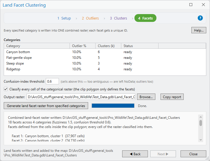
Land Facet Clustering, page 4 Facets: categories Canyon bottom 10 percent outliers 6 clusters ready, Flat-gentle slope 5 ready, Steep slope 3 ready, Ridgetop 4 ready; confusion-index threshold 0.6; Classify every cell of the categorical raster checked; output raster Land_Facet_Clusters in Test_Data.gdb; Generate button with progress bar Done; report beginning Combined land-facet raster written, 18 facets across 4 categories, Facets defined from the cells inside the clip polygon; every cell of the raster classified into them
All four classes ready, and the facet raster written: 18 facets across four categories. Leave Classify every cell of the categorical raster checked: the facets are defined from the cells inside the blocks, but every cell of the landscape is then assigned to one, which the density, diversity and cost surfaces of the next steps depend on.
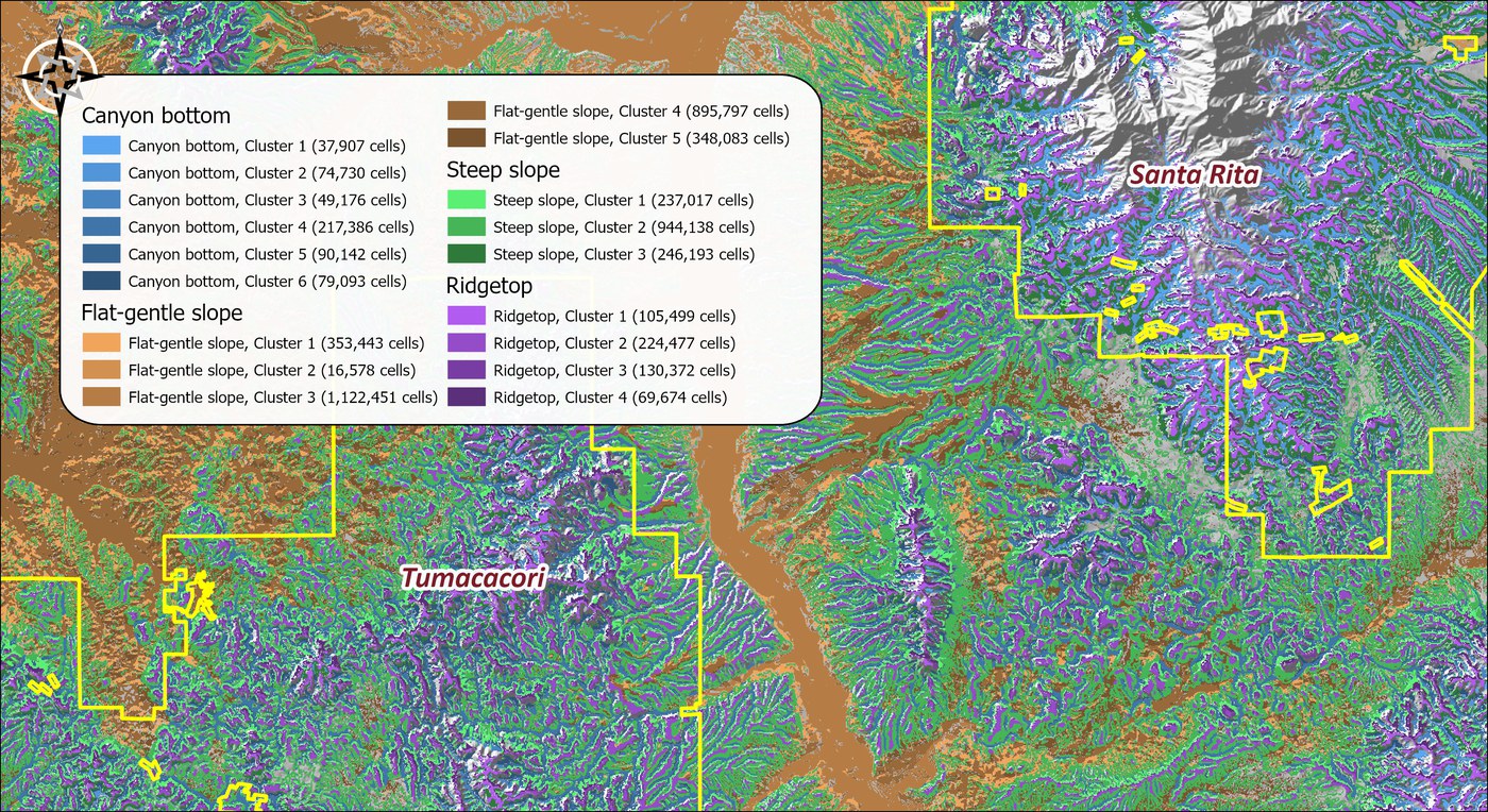
The land facet raster over a hillshade across the whole landscape: canyon-bottom facets in blues, flat-gentle-slope facets in browns, steep-slope facets in greens and ridgetop facets in purples, with the wildland blocks outlined in yellow and a legend giving each facet's name and cell count
The eighteen land facets, one color family per topographic position. They were defined from the cells inside the two blocks, but the whole landscape has been classified into them, so the valley between the blocks is mapped as well: mostly the big flat-gentle facets in brown, threaded by canyon-bottom and ridgetop facets along the drainages. The cells left unclassified are the outliers and the cells too confused between two facets, which show the hillshade through them.

Step 3: Density, then a cost surface per facet

Land Facet Density computes, for every cell and every facet, the proportion of the surrounding neighborhood occupied by that facet — one band per facet, eighteen bands here, in a single run. It reads the facet list from the raster's analysis record, so the dialog needs only the facet raster, an output name and a neighborhood.
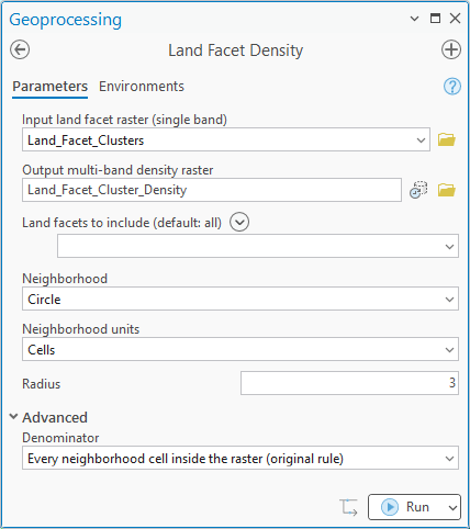
The Land Facet Density geoprocessing pane: input land facet raster Land_Facet_Clusters, output multi-band density raster Land_Facet_Cluster_Density, land facets to include left empty for all, neighborhood Circle, units Cells, radius 3, denominator Every neighborhood cell inside the raster (original rule)
Land Facet Density on the facet raster: all facets, a 3-cell circular neighborhood (100 m, the radius of the original work), and the original denominator rule.

Be warned that the result looks bizarre when it first appears on the map. A raster with many bands is drawn by ArcGIS as an RGB composite of its first three, so what you see is the first three canyon-bottom facets glowing in red, green and blue on black, and nothing of the other fifteen. The data are fine. To look at any one facet's density, change the layer's symbology from RGB to a single-band stretch and choose that facet's band.
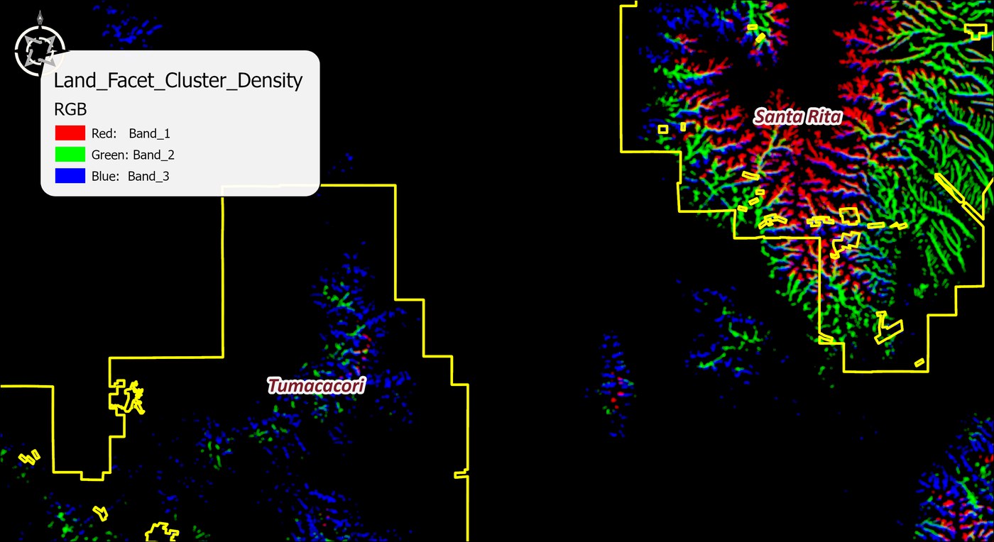
The density raster as ArcGIS first draws it: an RGB composite of bands 1, 2 and 3 on a black background, glowing blobs concentrated in the Santa Rita block with the wildland blocks outlined in yellow
The density raster as first drawn: bands 1, 2 and 3 as red, green and blue. Fifteen more bands are in there, unseen.

Then Land Facet Mahalanobis turns each facet into a cost surface: it samples the facet's characteristic values (the continuous rasters that produced the original land facet clusters, plus optionally the multi-band land facet density raster) from the wildland blocks, pins the density ideal at 100%, and computes the Mahalanobis distance of every cell in the analysis area from that ideal. Low distance = ground most like the facet at its best = cheap to cross; the D² output is already a valid cost surface, ready for corridor modeling with no inversion. The two tools validate each other's provenance records — a density raster from a different clustering run is refused, not warned about, because a wrong band produces plausible-looking nonsense.
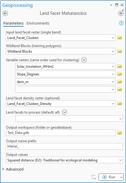
The Land Facet Mahalanobis geoprocessing pane: input land facet raster Land_Facet_Clusters, Wildland Blocks as training polygons, variable rasters Solar_Insolation_WHm2, Slope_Degrees and dem_m in the clustering order, land facet density raster Land_Facet_Clusters_Density, land facets to process empty for all, output workspace Test_Data.gdb, output name prefix Mahal_, output values Squared distance D2
Land Facet Mahalanobis: the facet raster, the blocks, the three variables in clustering order, the density raster, and a workspace and prefix for the eighteen outputs.
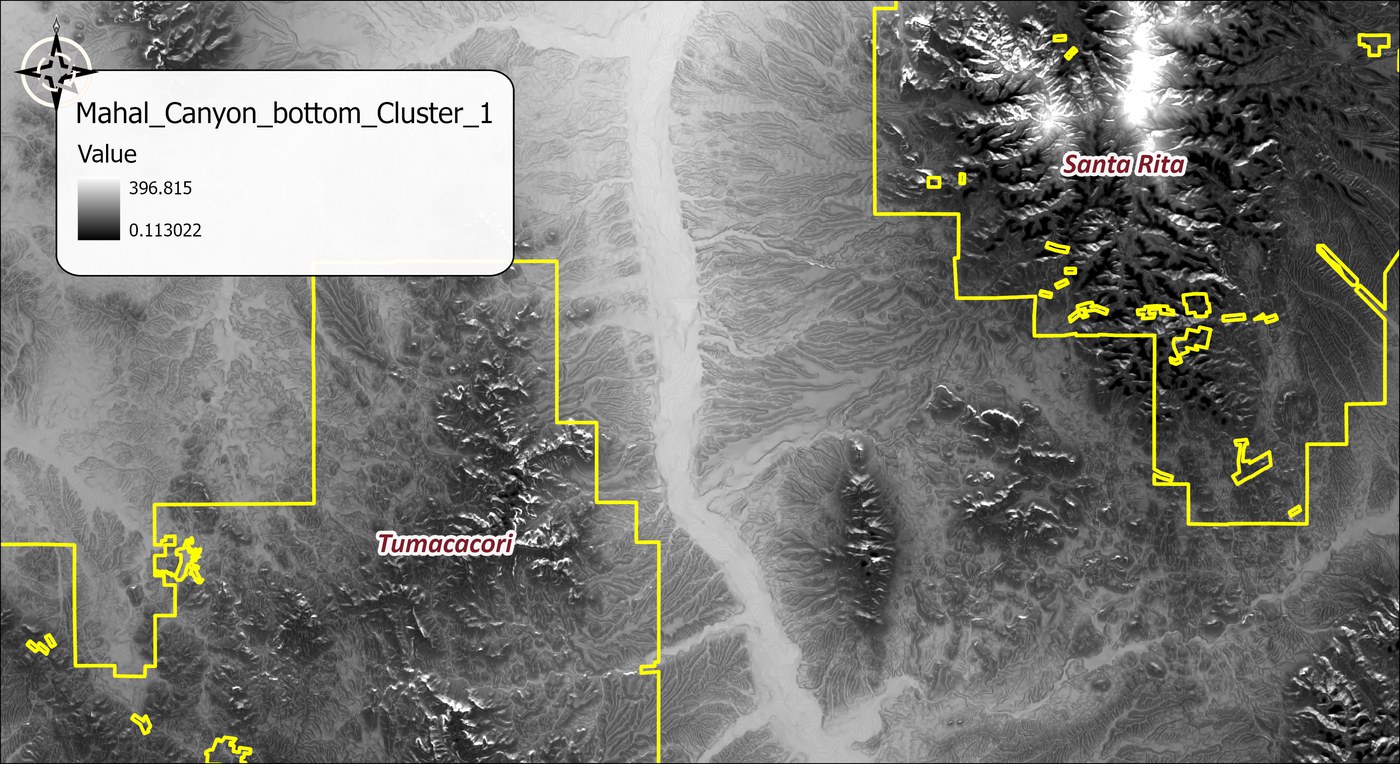
One of the eighteen Mahalanobis cost surfaces, for Canyon bottom cluster 1, as a gray stretch from 0.11 in black to 397 in white over the whole landscape: the drainage bottoms dark, the high Santa Rita peaks bright white, the wildland blocks outlined in yellow
One of the eighteen cost surfaces, Canyon bottom, cluster 1: dark where the ground is most like the facet and cheapest to cross, white where it is least like it, here the high Santa Rita peaks. There are seventeen more, one per facet, each cheap on its own kind of ground.

Step 4: A corridor per facet

Eighteen facets would mean eighteen rounds of termini and corridor modeling by hand. Both tools do all of them in one pass. Identify Termini Polygons takes the multi-band density raster and the wildland blocks, and for every facet converts the cells with any density at all (a fixed threshold of zero) into polygons, keeping in each block those at least half the size of the block's largest. The output is one feature class with a category per facet.
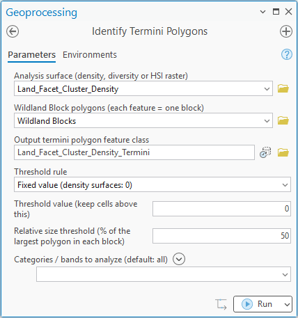
The Identify Termini Polygons geoprocessing pane for the land facet run: analysis surface Land_Facet_Cluster_Density, Wildland Block polygons Wildland Blocks, output Land_Facet_Cluster_Density_Termini, threshold rule Fixed value (density surfaces: 0), threshold value 0, relative size threshold 50 percent, categories to analyze left empty for all bands
Identify Termini Polygons on the density raster: threshold zero, 50% relative size, every facet.
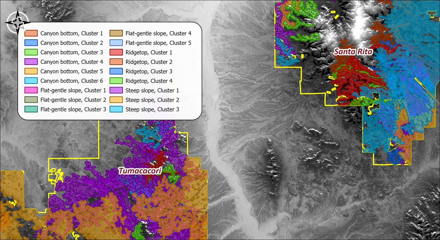
Termini polygons for all eighteen facets over a hillshade, one color per facet, filling much of both wildland blocks: the Tumacacori block dominated by steep-slope and flat-gentle-slope termini in purple and orange, the Santa Rita block by canyon-bottom, steep-slope and ridgetop termini in blues, red and green, with the block outlines in yellow
The termini: 101 polygons for 18 facets, filling much of both blocks. The crowding is expected; the corridor tool merges each facet's termini within a block.

Least-Cost Corridor is the same tool that built the species corridors in the Corridor Design Tutorial, and it handles the land facet case by being given two things instead of one: the termini feature class, with its category for every facet, and the geodatabase that holds the eighteen Mahalanobis surfaces. The tool pairs each facet's termini with its own cost surface through the information the earlier tools stored in the metadata, accumulates cost from both ends over that surface, and cuts the corridor at every percentile threshold in the list. The original guidance aims for strands roughly 1 km wide (2 km for long corridors); the tutorial carries the 1% slice forward, about 5,700 hectares per facet.
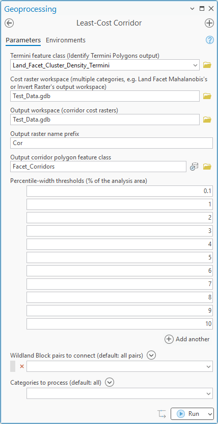
The Least-Cost Corridor geoprocessing pane for the land facet run: termini feature class Land_Facet_Cluster_Density_Termini, cost raster workspace Test_Data.gdb, output workspace Test_Data.gdb, output raster name prefix Cor, output corridor polygon feature class Facet_Corridors, percentile-width thresholds 0.1 and 1 through 10 percent of the analysis area, Wildland Block pairs and categories left at all
Least-Cost Corridor for all eighteen facets: the termini feature class, the geodatabase of Mahalanobis surfaces as the cost workspace, and the default percentile slices.
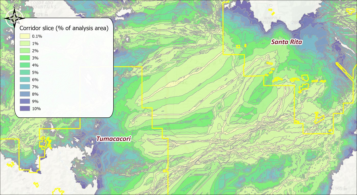
Every corridor slice of every facet drawn at once over a topographic base: nested bands from pale yellow at 0.1 percent through greens to blue-violet at 10 percent, covering nearly the whole landscape between and around the two wildland blocks outlined in yellow
Everything the run produced, drawn at once: eleven nested slices for each of eighteen facets, 209 polygons. Not a useful map, but a fair picture of what the corridor tool hands back.

To see the strands themselves, keep one slice per facet. The output has a Percentile field, so a definition query on the layer does it without touching the data: open the layer's properties, add a definition query, and set Percentile is equal to 1.
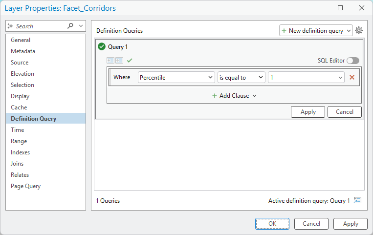
The Layer Properties dialog for Facet_Corridors on the Definition Query page, with one query: Where Percentile is equal to 1
A definition query keeps only the 1% slice of every facet on the map.
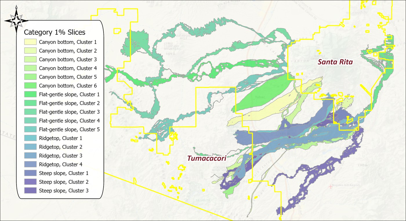
The 1 percent slice of each of the eighteen facet corridors, one color per facet: flat-gentle-slope strands in greens looping far to the north of the Tumacacori block around the Cerro Colorado and Batamote hills, canyon-bottom strands in pale yellows and greens crossing the valley near Tubac, ridgetop and steep-slope strands in blues running southeast along the mountains and south past the Nogales airport, with the wildland blocks outlined in yellow
The eighteen 1% strands, one color per facet. Each is the same area, about 5,700 hectares, but they go where their own kind of ground goes: the flat-gentle strands loop north around the hills, the canyon-bottom strands cross the valley near Tubac, and the ridgetop and steep-slope strands follow the mountains southeast and south. This spread is the point of the method. No single corridor could serve all of these facets, and a linkage that keeps a strand of each one keeps a route for whatever will depend on it.

A word on what these strands are for. They are defined by terrain, and nobody expects a “flat-gentle slope” to get up and cross the landscape. But the expectation behind the method is that animals will use these corridors, now and under whatever climate comes, so it is fair to ask of each strand what one would ask of a species corridor. Any of the standard evaluation tools in the Corridor Evaluation Tutorial can be run on a facet strand: Bottleneck Analysis to find where it pinches, or Weighted Summary Statistics and Cross-Tab Statistics for what it crosses. If a strand turns out too narrow to be useful, or so wide it says nothing, a different percentile slice is the remedy, and the corridor tool has already cut them. This tutorial keeps the 1% slice for every strand for simplicity's sake.

Step 5: The interspersion corridor

One more corridor rewards variety rather than any single facet — ground where many facets interleave supports range shifts and species turnover as climate moves. Run Diversity Indices on the facet raster with Shannon's H′ in a 5-cell circle, the original work's 5-pixel radius. The tool's default measure is the effective number of species, the more interpretable index and the one to prefer for reporting diversity, but it is simply exp(H) and ranks every cell the same way; the tutorial picks Shannon's H so that the next step can reproduce the published resistance formula exactly.
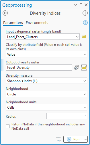
The Diversity Indices geoprocessing pane: input categorical raster Land_Facet_Clusters, Classify by attribute field left at Value, output diversity raster Facet_Diversity, diversity measure Shannon's Index (H), neighborhood Circle, units Cells, radius 5, and the Return NoData if the neighborhood includes any NoData cell box unchecked
Diversity Indices on the facet raster: Shannon's index in a 5-cell circle.
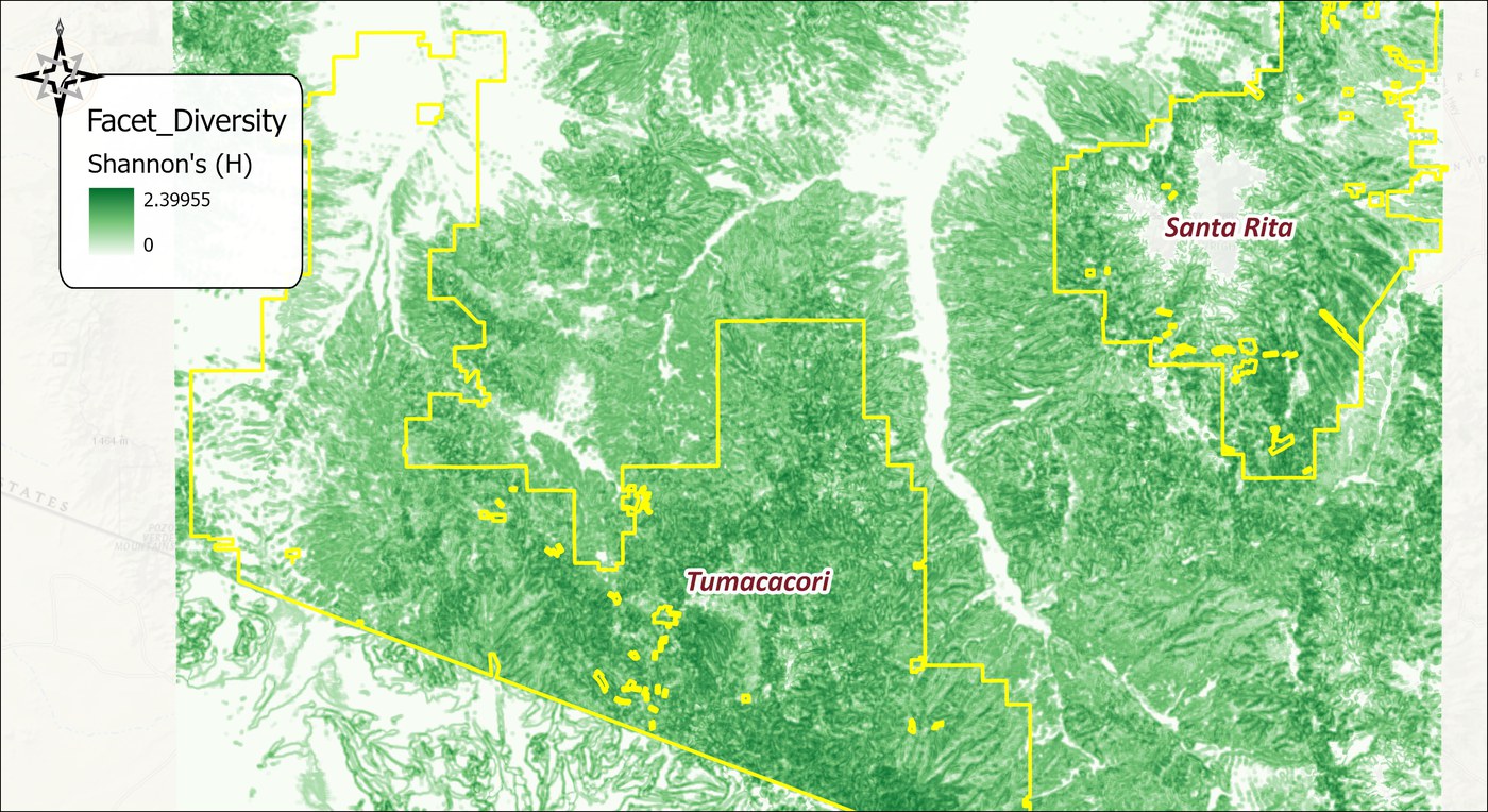
Shannon diversity of land facets over the study area as a white-to-green ramp from 0 to 2.4: dark green where many facets interleave along the dissected hills and mountain fronts, white on the uniform valley floor, and a gray NoData hole at the high Santa Rita summit where the outlier cells were excluded, with the wildland blocks outlined in yellow
Facet diversity, 0 to 2.4. The dissected hills and mountain fronts are dark green, where many facets meet within 150 m; the valley floor is white, one facet as far as the window reaches. (The gray hole at the Santa Rita summit is not low diversity but NoData: the cells the clustering excluded as outliers, which carry no facet.) This is the ground the interspersion corridor will seek out and the ground it will avoid.

Then invert it with Invert Raster. We consider high land facet diversity to be better than low, and yet we want to use the surface as a cost surface, where low is good, so the diversity values have to be inverted: high diversity must become low cost. The tool's 1/(x + c) mode with c = 0.1 reproduces the original 1/(H′ + 0.1) formula.
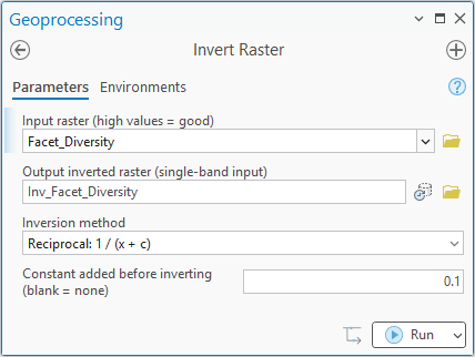
The Invert Raster geoprocessing pane: input raster Facet_Diversity, output inverted raster Inv_Facet_Diversity, inversion method Reciprocal 1 divided by x plus c, constant added before inverting 0.1
Invert Raster on the diversity surface: reciprocal, constant 0.1.
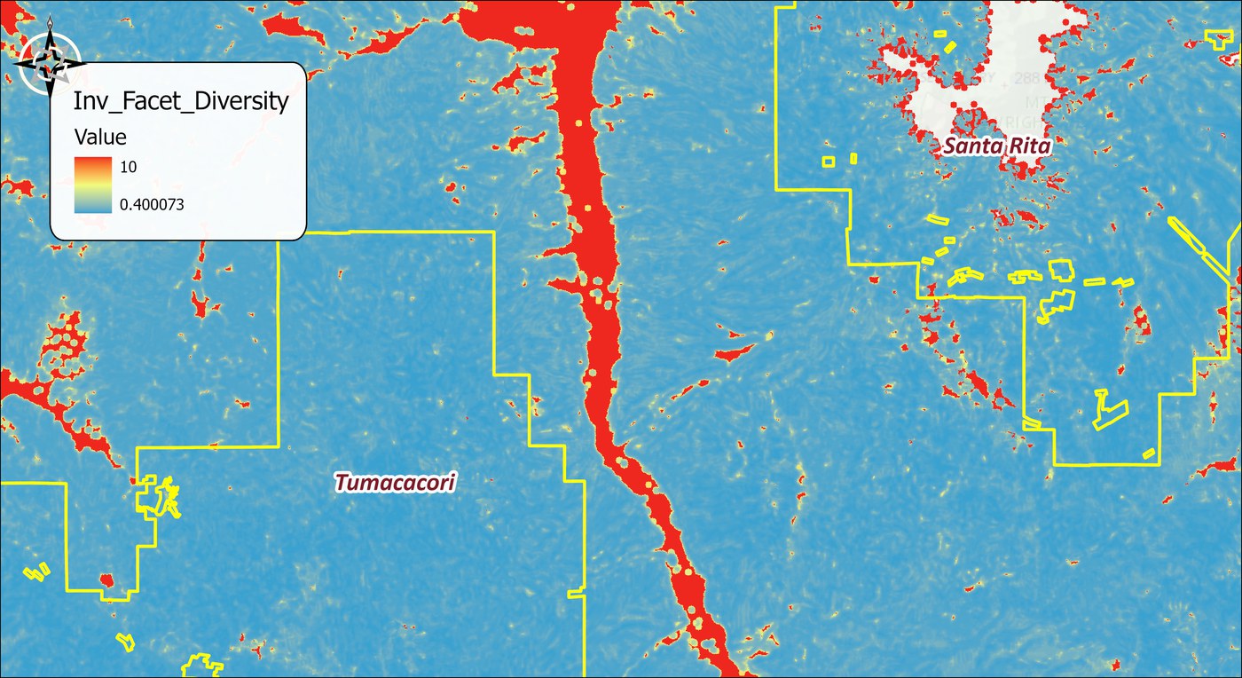
The inverted diversity surface as a cost raster, blue at 0.4 through yellow to red at 10: blue over the dissected hills and mountain fronts, red along the flat floor of the Santa Cruz valley, and in scattered patches of uniform ground, with a gray NoData hole at the high Santa Rita summit and the wildland blocks outlined in yellow
The interspersion cost surface, 0.4 to 10. The diverse hills are now cheap and blue; the uniform valley floor along the Santa Cruz is a red wall of cost. The corridor will have to find a way across that floor.

Now take termini from the high-diversity concentrations in each block. The analysis surface is the diversity raster itself, not the inverted one, and the threshold rule is median within each Wildland Block this time, since a diversity surface has no natural zero to threshold at; the 50% relative size test is the same as before.
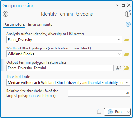
The Identify Termini Polygons geoprocessing pane for the diversity run: analysis surface Facet_Diversity, Wildland Block polygons Wildland Blocks, output Facet_Diversity_Termini, threshold rule Median within each Wildland Block (diversity and habitat suitability surfaces), relative size threshold 50 percent
Identify Termini Polygons on the diversity surface: the median-within-block rule, which needs no threshold value, and the same 50% size test.
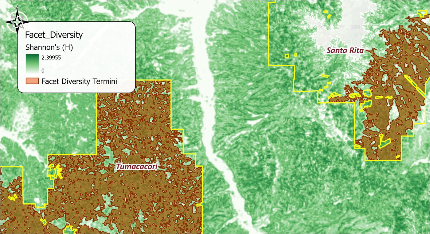
The diversity termini over the Shannon diversity surface: one large brown terminus polygon filling most of the Tumacacori block and another filling the southern half of the Santa Rita block, each riddled with small holes where diversity falls below the block median, with the wildland blocks outlined in yellow
The diversity termini, from Identify Termini Polygons with the median within each Wildland Block rule: in each block, the cells above that block's median diversity, joined into regions, of which only the largest half survive. One terminus per block, each a broad mass of diverse ground pocked with holes where a single facet dominates.

Then run the least-cost corridor exactly as in Step 4, with one difference: instead of a workspace of cost surfaces, give it the inverted raster as the single cost surface.
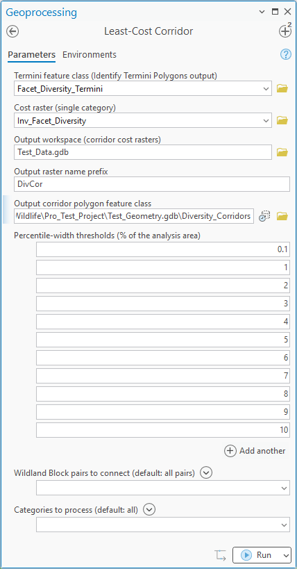
The Least-Cost Corridor geoprocessing pane for the diversity run: termini feature class Facet_Diversity_Termini, cost raster Inv_Facet_Diversity as a single category, output workspace Test_Data.gdb, output raster name prefix DivCor, output corridor polygon feature class Diversity_Corridors, the default percentile thresholds, block pairs and categories left at all
Least-Cost Corridor for the interspersion strand: the diversity termini and the inverted diversity raster as a single cost surface, everything else as in Step 4.
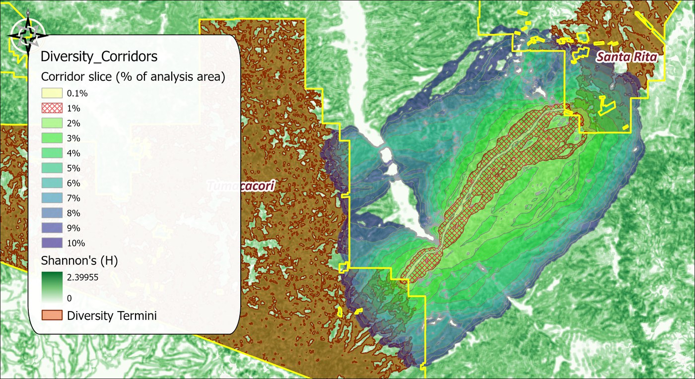
The interspersion corridor between the two wildland blocks over the diversity surface: nested slices from 0.1 to 10 percent, the 1 percent slice cross-hatched in red running from the eastern edge of the Tumacacori block northeast to the southern part of the Santa Rita block, crossing the Santa Cruz valley floor at its narrowest, with the diversity termini in brown filling the blocks
The interspersion corridor, all slices, with the 1% slice cross-hatched. It leaves the Tumacacori block on its eastern edge, crosses the uniform valley floor where that red wall of cost is narrowest, and climbs through the dissected foothills into the Santa Rita block. Unlike the facet strands, it follows no single kind of ground; it follows the seams between kinds.

Step 6: Join the strands

The strands now live in two feature classes: Facet_Corridors, holding every percentile slice of all eighteen facets, and Diversity_Corridors, holding the slices of the interspersion corridor. The linkage design is the union of one slice from each, not of everything, so before running Union Corridors the 1% slices have to be picked out. Either of two ways works: a definition query on each layer, as in Step 4, or a selection. The tool honors a layer's selection, so selecting the 1% slices with Select By Attributes on both layers is enough; the dialog then shows the count it will use under each input.
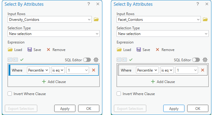
Two Select By Attributes dialogs side by side: Diversity_Corridors and Facet_Corridors, each with a new selection where Percentile is equal to 1
Select By Attributes on both corridor layers: Percentile is equal to 1, one polygon in the diversity layer and eighteen in the facet layer.
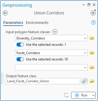
The Union Corridors geoprocessing pane: input polygon feature classes Diversity_Corridors with Use the selected records 1, and Facet_Corridors with Use the selected records 18; output feature class Land_Facet_Corridor_Union
Union Corridors with the two selected layers: one diversity polygon and eighteen facet polygons, into one output. A hand-drawn riverine strand would be a third input here if the landscape needed one.
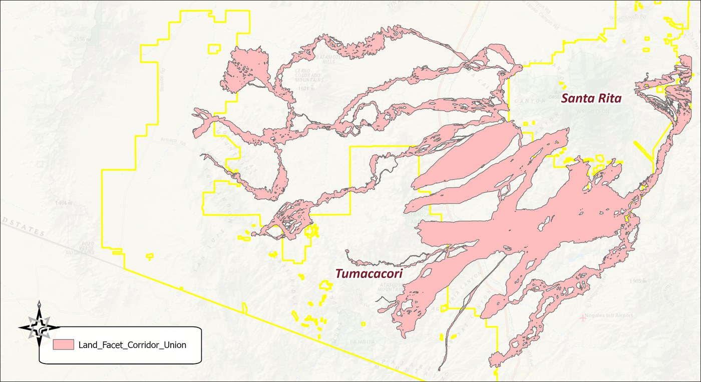
The unioned linkage design in pink over a topographic base: the nineteen 1 percent strands merged into one polygon that sprawls from the Tumacacori block north around the Cerro Colorado and Batamote hills, across the valley to the Santa Rita block, and south along the mountains toward Nogales, with many small holes and slivers, and the wildland blocks outlined in yellow
The preliminary linkage design: nineteen strands merged into one polygon of about 72,000 hectares. It reaches north around the hills, across the valley and south along the mountains, because that is where the facets went, and it is full of small holes and slivers where strands crossed and missed each other.

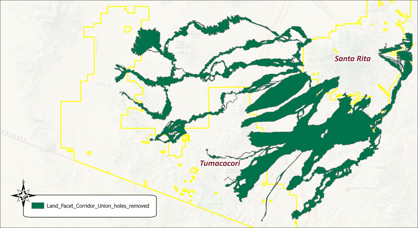
Fill Corridor Holes closes the gaps that mean nothing. The threshold is a judgment about the landscape: here 25 hectares, so that rasterization slivers and the small islands between crossing strands are filled while any real opening larger than that is kept for a decision.
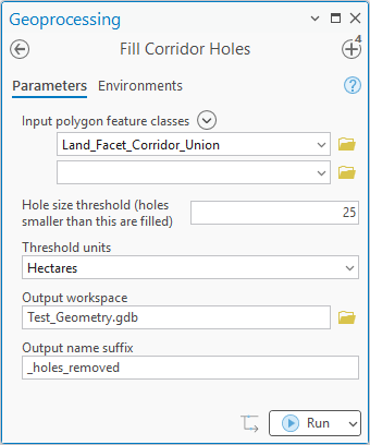
The Fill Corridor Holes geoprocessing pane: input polygon feature class Land_Facet_Corridor_Union, hole size threshold 25, threshold units Hectares, output workspace Test_Geometry.gdb, output name suffix _holes_removed
Fill Corridor Holes on the union: holes under 25 hectares filled.
The linkage design after filling, in dark green: the same sprawl of strands with the small holes and slivers closed, only the larger openings kept, with the wildland blocks outlined in yellow
The linkage design with the small holes filled: the strands read as solid ground, and only the larger openings remain.

Two things finish the job. Cumulative Surface counts how many strands cover each cell, and the ground that serves many facets at once is the heart of the linkage, the part to protect first. And the Corridor Analysis Data Report window will recount the whole chain — every input, parameter and ancestor — from the provenance records the tools have been stamping all along.
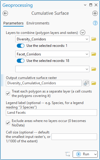
The Cumulative Surface geoprocessing pane: layers to combine Diversity_Corridors with Use the selected records 1 and Facet_Corridors with Use the selected records 18; output Diversity_Cumulative_Corridors; Treat each polygon as a separate layer checked; legend label Land Facets; Exclude areas where no layers occur checked; cell size blank
Cumulative Surface on the same two selected layers. Treat each polygon as a separate layer is what makes the eighteen selected facet slices count as eighteen strands rather than one layer; the empty ground is set to NoData so only the design draws.
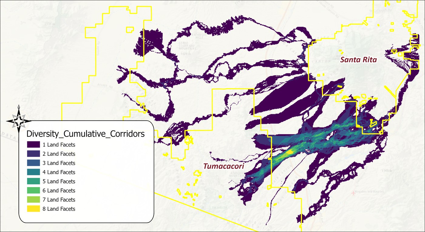
The cumulative surface of the nineteen strands over a topographic base, from dark purple where one land facet strand covers a cell through blue and green to yellow where eight overlap: most of the sprawling design is a single strand, and the overlap concentrates in one band running from the Tumacacori block northeast across the Santa Cruz valley toward the Santa Rita block, with the wildland blocks outlined in yellow
How many strands cover each cell, one to eight. Most of the design is a single strand, ground that serves one facet and no other. The overlap gathers in one band from the Tumacacori block northeast across the valley toward Santa Rita, where up to eight strands, the interspersion corridor among them, want the same ground. If the design has a core, that is it, and it is the part to protect first.

Recommended citation

Jenness, J., B. Brost and P. Beier. 2026. Corridor Designer Tools. Wildlife and Forestry Tools add-in for ArcGIS Pro, v. 1.99 (September 2026). Jenness Enterprises. Available at: https://github.com/JeffJenness/Wildlife_Tools.

Credits and references

The land facet methodology is by Paul Beier and Brian Brost; the original tools and these ArcGIS Pro ports are by Jeff Jenness with Brost and Beier, produced with the support of the USDA Forest Service Rocky Mountain Research Station and the Arizona Board of Forest Research / McIntire-Stennis Cooperative Forestry Program.