

About Topographic Roughness
Just what is it, anyway?
Everyone has an intuitive sense of what rugged terrain looks like, and many wildlife species clearly respond to it: bighorn sheep are famous for traversing horrendously rugged terrain, pronghorn and elephants are famous for preferring gentle topography, and mule deer and white-tailed deer may partition habitat partly by how rugged it is (Kramer 1972, as cited by Beasom et al. 1983). The trouble starts when you try to put a number on it. Topographic roughness (or ruggedness; I use the two words interchangeably) is not one well-defined quantity. Depending on the question you are asking, it might mean any of the following:
- Variation in elevation — how much the elevations in a neighborhood differ from one another, or from the cell in the middle.
- Steepness — slope, or the closely related idea of how much extra land surface a cell contains because it is tilted.
- Curvature — how bent the surface is: peaks, pits, ridges and drainages, which has direct effects on hydrologic flow and on how exposed vs. protected a location is.
- Variation in direction — whether neighboring cells all face the same way or face every which way.
- Rippling — repeating waves in the surface, such as sand dunes, seabed ripples or a washboard road.
- Fractal dimension — how the amount of detail keeps growing as you look more closely.
There is no right answer among these, only measures that are appropriate for different questions. A landscape ecologist interested in the amount of habitat available to a population, a biologist modeling escape terrain, and a hydrologist worried about where water accelerates all want different metrics, and all three of them are entitled to call their metric roughness. The nine tools in the Topographic Roughness menu implement a variety of different approaches that I have found useful, and this page is meant to help you pick among them. It follows the Topographic Roughness lecture from my GIS course (slides), which walks through the same ideas with more pictures; see the training page for the course itself.
The nine tools at a glance
Six of the tools take a DEM and produce a raster in which every cell holds a roughness value for the neighborhood around it; LSRI on Contours does the same from a contour feature class instead of a DEM. The last two take polylines and a DEM, because sometimes the question is not how rough the landscape is but how rough a particular route through it is.
| Tool | What it measures | Output and range |
|---|---|---|
| Surface Area and Ratio | The true three-dimensional area of the terrain in each cell (Jenness 2004), and its ratio to the flat map area. Steep or convoluted cells contain more surface. | Area in the units you choose; ratio from 1 (flat) upward, rarely above 2 or 3. |
| Vector Ruggedness Measure (VRM) | How much the directions the cells face vary within a neighborhood (Sappington et al. 2007). A steep but even slope scores the same as flat ground. | 0 (all cells face the same way) to 1 (maximum dispersion). |
| Arc-Chord Ratio (ACR) | Surface area divided by the area of the cell's tilted plane of best fit rather than its flat footprint (Du Preez 2015), so a smooth tilted plane scores 1. | 1 (flat or smoothly sloped) upward. |
| Terrain Ruggedness Index (TRI) | How much the neighboring elevations differ from the focal cell (Riley et al. 1999; Wilson et al. 2007), from the neighborhood mean, or, in a variant of my own, the slopes to the neighbors. | Elevation units (meters or feet), or a unitless rise-over-run for the slope variant; 0 upward. |
| Fractal Dimension | How the roughness inside a window changes with the scale you measure it at (Clarke 1986; Gneiting et al. 2012). | 2 (a smooth surface, tilted or not) to 3 (a surface so convoluted it fills space). |
| LSRI on DEM | The total length of contour line within a circle around each cell, with the contours traced from the DEM on the fly (Beasom et al. 1983). | Length in the units you choose; 0 upward. |
| LSRI on Contours | The same index computed from contour lines (or any polylines) you already have. | Length in the units you choose; 0 upward. |
| Topography along Lines | Roughness of a route rather than a landscape: surface length, climbing and descending, slope statistics, direction statistics, sinuosity and fractal dimension of each polyline, written as attribute fields. | One field per statistic, each in its own stated units. |
| Split Lines into Topography Segments | The same lines broken into their straight three-dimensional segments, each with its own slope, bearing and turning angles, for symbolizing or summarizing yourself. | A new PolylineZ feature class. |
Three generations of ruggedness index
Dilts et al. (2023) presents a clever way to organize these measures, by sorting the ruggedness indices in the ecological literature into three generations according to three simple tests, which they call the criteria for an ideal ruggedness index. The first test is a smooth, tilted plane: a hillside with no bumps on it at all. Should it count as rugged? To pass this test means to give that smooth hillside the same score as flat ground: the index should respond to bumps, not to tilt, so that steepness and ruggedness can be measured as two separate things. The second test is a smooth fold, such as a rounded ridgeline or the bottom of a gentle drainage, where adjacent cells face different directions even though the surface itself is perfectly smooth. To pass this test means to give that smooth fold a low score too: the index should not mistake a change of direction for roughness, so that a rounded ridge scores like the smooth slopes on either side of it and only a genuinely bumpy surface scores high. The third test is the one every index ought to pass: take a rough surface and exaggerate its relief, doubling it and doubling it again. To pass this test means that the score rises each time, because the surface really is getting rougher. All six of the indices they tested pass it (the surface ratio, ACR and VRM, each with and without detrending), so it is the first two tests that separate the generations.
First-generation indices measure variation in elevation, and they fail the tilted-plane test: a smooth steep hillside has elevations that genuinely differ across it, so it scores as rugged. The surface ratio, the Terrain Ruggedness Index, the standard deviation of elevation and the Land Surface Ruggedness Index all belong here. That is a fault only if you did not want steepness included. If your animal experiences a steep smooth slope as difficult terrain, a first-generation index is the right choice, and both Riley et al. (1999) and Beasom et al. (1983) defined ruggedness to include elevation change.
Second-generation indices measure variation in aspect and gradient together, and they pass the tilted-plane test. On a smooth slope every cell faces the same way, so the Vector Ruggedness Measure scores it near zero, exactly like flat ground; only terrain that is both steep and broken scores high. Sappington et al. (2007) built VRM for precisely this reason, so that slope and ruggedness could enter a bighorn sheep habitat model as two separate variables. The Arc-Chord Ratio gets the same independence from slope a different way, by measuring surface area against a tilted reference plane. Both, however, still fail the smooth-fold test: a rounded ridge reads as rugged simply because the cells on either side of it face opposite directions.
Third-generation indices measure local surface roughness itself, and pass all three tests. The recipe of Dilts et al. is simple: smooth the DEM with a small neighborhood mean, subtract that smoothed surface from the original to leave only the fine-scale bumps, and then run an ordinary index on the residual. They call the results the local variants (VRM-L, SAPR-L and ACR-L), and report that these “did a better job of mapping rugged terrain, such as rock outcrops and cliff bands” (p. 1405) and “tended to modestly improve habitat models” for bighorn sheep relative to the uncorrected versions (p. 1403).
To be clear, the three generations are not simply better and worse. Some phenomena really do treat a steeply sloped plane as more rugged than a horizontal one, and some treat a smooth fold as more rugged than a flat surface. Elephants and pronghorn will choose the horizontal plane over the steep slope no matter how smooth that slope is, so there is a place for first- and second-generation measures. But the third generation gets at a genuinely distinct kind of roughness, and it captures fine-scale roughness better than the earlier measures. Picture a steep hillside of smooth grass next to a talus field of the same steepness, with a rounded ridge crest above them both. A first-generation index scores all three as rugged, because all three are steep or high. A second-generation index correctly separates the grass from the talus, but it also flags the smooth crest as rugged, because the cells on its two sides face different ways. Only the third-generation index scores the talus alone. That is the kind of surface Dilts et al. (2023, p. 1406) have in mind when they write that third-generation metrics may indicate “surface features such as boulder patches, which may be critical for certain species.”
Dilts et al. (2023) saw exactly this difference across several hundred Nevada mountain ranges. Looking at the most rugged tenth of cells, switching from VRM to VRM-L cut the number on drainages by 45% and on ridges by 46%, and raised the number on mid-slopes by 59% (p. 1403). In their desert bighorn sheep case study the ewes selected steep slopes at fine scales and ruggedness at moderate scales. In this toolbox the third generation is not a separate tool. The Surface Area, VRM and ACR tools each offer a Remove smooth topography first option that applies the Dilts detrending before computing the index, so from the same dialog you can produce the first- or second-generation measure or its third-generation local variant, and apply whichever generation suits your question.
Fractal dimension sits a little apart from this scheme. It passes the tilted-plane test (a tilted plane is still a plane, with a dimension of exactly 2), but it measures something different from all of the above: not how rough the surface is at one neighborhood size, but how the roughness grows as the neighborhood shrinks.
Roughness and slope: the central-cell problem
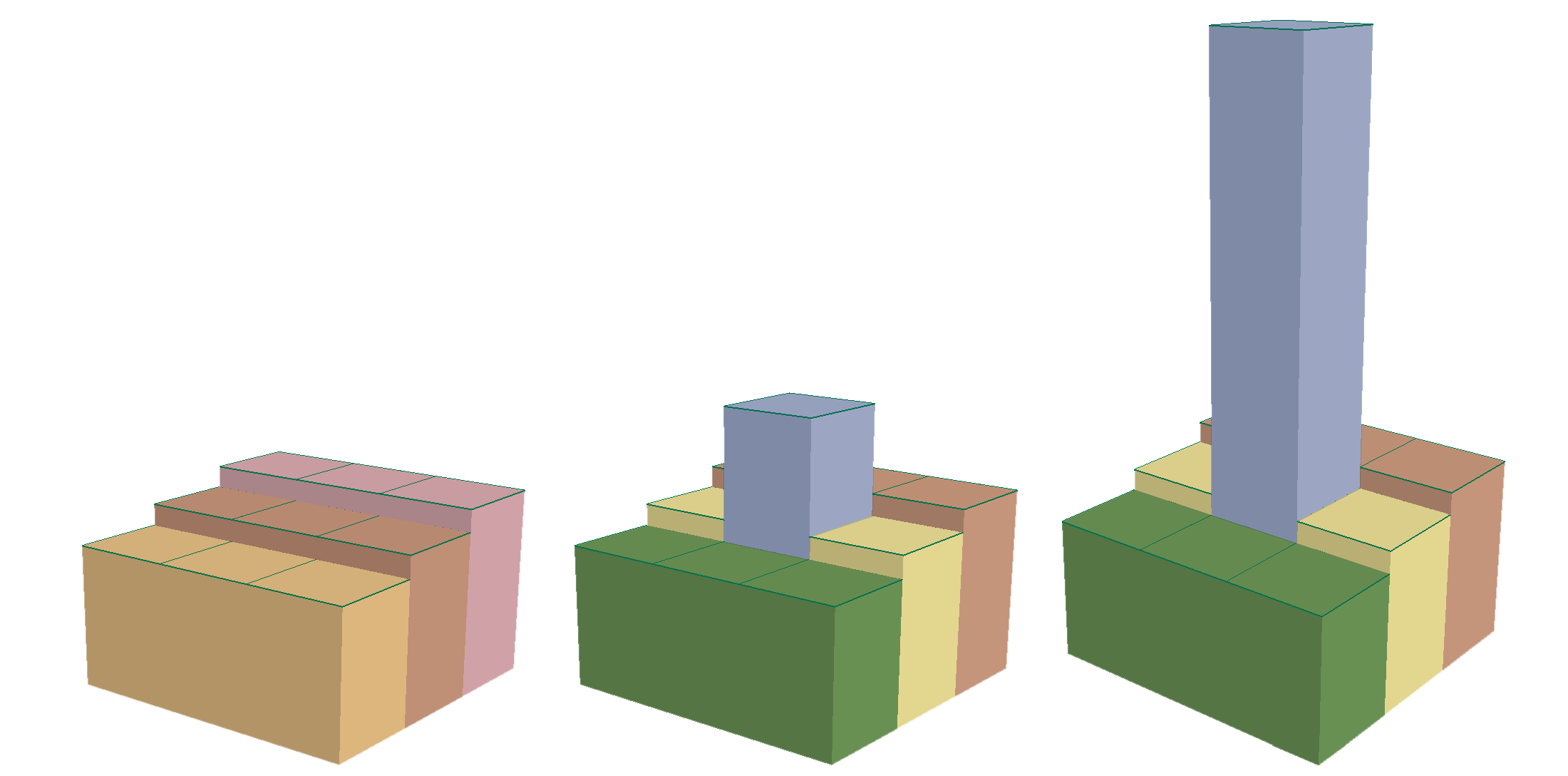
Slope is the simplest roughness measure of all, and often a perfectly good one. But two things about slope are worth knowing before you use it, or anything derived from it, as a roughness index. First, many slope algorithms (Jones 1998 compares eight of them) never use the elevation of the cell whose slope they are computing. Horn's method (Horn 1981), which the ArcGIS Pro Slope tool uses, takes an east-west gradient from the six cells in the left and right columns and a north-south gradient from the six cells in the top and bottom rows; the central cell contributes nothing. That is fine for slope, which really is a property of the surrounding surface, but it means a spike or a pit in the middle of a neighborhood is invisible. The three neighborhoods above have identical slopes, and the two on the right below are all perfectly flat as far as the algorithm is concerned.
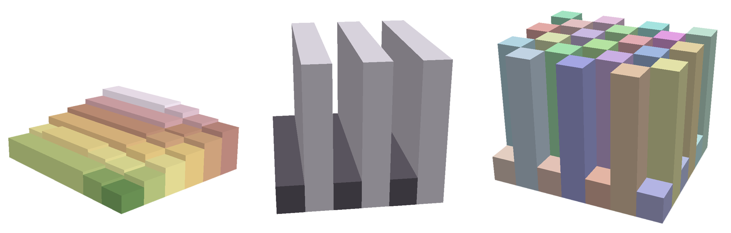
Second, Hodgson (1995) showed, on a mathematical surface where the true slope was known everywhere, that most algorithms return a slope representing an area 1.6 to 2 times the size of the cell. The slope value for a cell therefore describes a slightly larger patch of ground than the cell itself, which smooths the landscape a little. Neither point matters much for slope as a habitat variable. They matter a great deal if you derive surface area from slope by dividing the cell area by the cosine of the slope angle (the cosine method described by Berry 2002), because that estimate will be too low wherever the central cell rises above or falls below the plane of its neighbors, which is to say almost everywhere. That is the reason the Surface Area and Ratio tool builds triangles through the central cell instead.
ArcGIS Pro's newer Surface Parameters tool takes a more advanced approach (see Esri's tool reference and its How Surface Parameters works page). Instead of Horn's fixed weights it fits a local surface to the neighborhood by least squares, either a quadratic surface (the default, which does not pass exactly through the cell centers and so smooths noisy data such as lidar) or a biquadratic surface (which passes through all nine cells exactly), and takes the slope as the first derivative of that fitted surface at the cell center. The neighborhood can be larger than 3 × 3, and an adaptive option shrinks it where the terrain is variable. That is a real improvement for curvature and for noisy high-resolution surfaces. It does not, however, cure the central-cell problem for slope, and the reason is geometry rather than any shortcoming of the tool: the neighborhood is symmetric about the cell being evaluated, so the central cell sits at the origin of the fitted surface, where it can push the surface up or down but cannot tilt it. Whatever its elevation, the first derivatives at the center come from the surrounding cells alone. A test of the tool on synthetic DEMs confirms this: raising the central cell of a smooth 5.7° ramp by 10 m or by 100 m left the quadratic slope at 5.71° and moved the biquadratic slope by 0.2° at most, and the parallel-ridge and checkerboard surfaces above came out at exactly 0° under both surface types, just as under Horn's method. What the central cell does change is the curvature: the same 10 m bump moved the profile curvature from zero to a clearly nonzero value. So if you want a slope-based measure that sees the central cell, a fitted surface will not give it to you; the eight-triangle Surface Area and ACR tools, which build their triangles from the central cell's elevation, and TRI, which compares it directly with its neighbors', will. VRM sees it only indirectly, through the Horn normals of the surrounding cells, each of whose 3 × 3 windows includes it.
Scale: the neighborhood is part of the answer
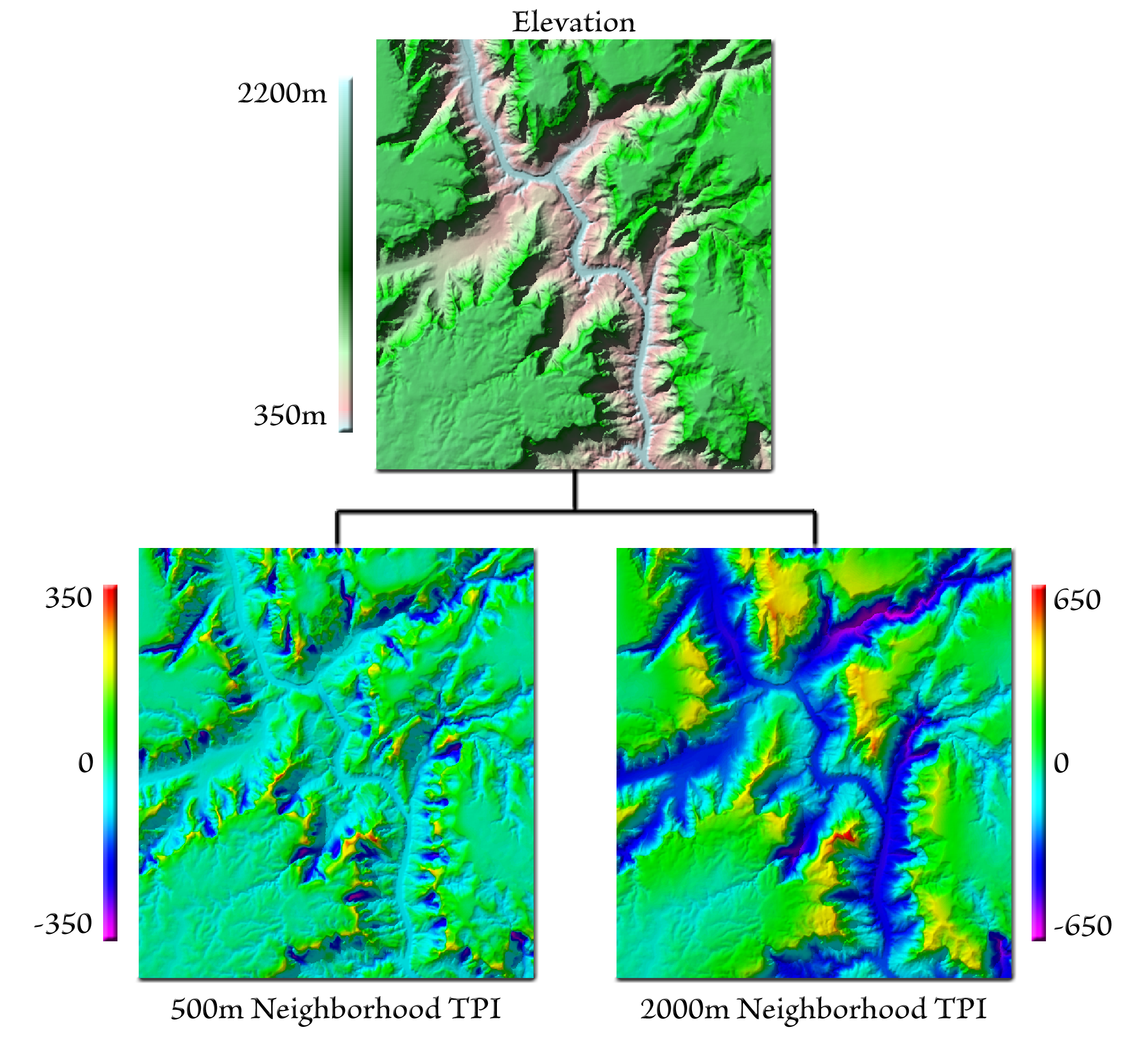
Every one of these indices is computed over some neighborhood of the cell: a 3 × 3 window, a circle of a radius you choose, or a square window of some width. That neighborhood is the scale of the analysis, and it is part of the definition of the number you get. What counts as rugged depends on the scale at which the organism or process experiences the terrain. The Grand Canyon is extremely rugged at a 2 km scale, and perfectly smooth at the scale of the flat bench a mule stands on. Luckhurst and Luckhurst (1978) showed the same thing with animals. They measured the rugosity of coral reefs by draping a chain over them, at the scale of what they called gross reef morphology, and found that the number of fish species larger than 50 mm was strongly related to it (r = 0.81) while the number of species smaller than 50 mm, for which the individual coral matters more, was not (r = 0.54, not significant). In their words, “the scale of the SR index may have a strong influence on the correlations.” (The chain method is described on the Arc-Chord Ratio page.) There is no universal right neighborhood, and I encourage you to run a tool at two or three radii and look at what each one shows you before settling on one. Sappington et al. (2007) chose a 3 × 3 window on a 30 m DEM for bighorn sheep, partly so that it covered an area comparable to the two indices they were comparing it with and partly because larger windows smoothed the terrain; Beasom et al. (1983) used 40-hectare circles and do not say why (it may have just been a practical size to trace on a paper map); Riley et al. (1999) worked with 1 km cells across the whole state of Montana. All three were sensible for their purposes and none of them is a rule.
A related point: the cell size of the DEM sets the finest scale any of these tools can see. Roughness that exists between the cell centers, such as a boulder field on a 30 m DEM, is simply not in the data. If two DEMs of the same terrain have different cell sizes, their roughness rasters will differ even with identical settings, and the coarser one will generally look smoother. Compare roughness values only between runs on the same DEM at the same settings.
Units, ranges and what not to compare
The indices report in different units, and the differences are not cosmetic. The surface ratio, ACR and VRM are unitless and have natural floors (1, 1 and 0), so they are comparable from one DEM to another if the cell sizes and neighborhoods match. TRI and the standard deviation of elevation are in the DEM's own elevation units, meters or feet, so a DEM in feet gives numbers 3.28 times larger than the same terrain in meters; Riley et al.'s published ruggedness classes (level, nearly level, slightly rugged and so on) assume meters and a 3 × 3 window. LSRI is a length, and it roughly doubles when you halve the contour interval, so it too is comparable only between runs with the same interval and radius. Fractal dimension is unitless and bounded between 2 and 3, but the several algorithms for estimating it give somewhat different values on real terrain, so pick one algorithm and stay with it.
The safest practice is to treat each index as a relative measure within one study: compute it once, on one DEM, with one set of settings, and compare locations within that raster. When you do need to compare across studies, match the DEM resolution, the neighborhood and the units, and say so in your methods.
Roughness along a line
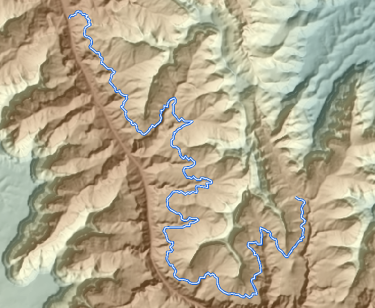
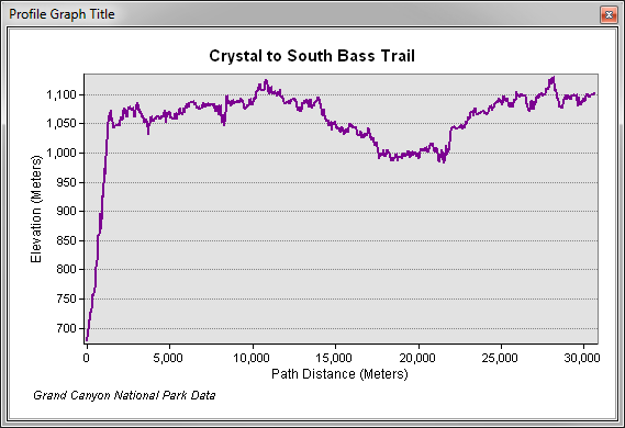
Remember your research question. If you are studying animal movement, the general roughness of the landscape may be only indirectly related to what the animal experiences. An animal that sticks to trails, game paths or drainages crosses the Grand Canyon on a route that is remarkably gentle, and a roughness raster of the canyon tells you little about that route. A GPS track of an animal, if its fixes are frequent enough, can tell you a great deal about how that animal actually traverses a rugged landscape, and that might be an interesting study in itself: observed path ruggedness against landscape ruggedness. For those questions the two line tools measure the route itself: how long it is on the ground versus on the map, how much of it climbs and descends, how steep and how variable the slopes are, whether it heads consistently in one direction, and how convoluted its path is. The segments tool goes one step further and hands you every straight piece of every line with its own slope and bearing, so that you can compute whatever summary you like or simply symbolize the uphill stretches in red.
Measures that live elsewhere
Two ideas from the lecture are not in this menu because they are better served by other tools. Curvature is a good measure of exposure and protection, and of whether water converges or accelerates as it crosses a cell, and ArcGIS Pro's own Surface Parameters tool computes profile, plan, tangential and total (Casorati) curvature very well. Topographic position, the difference between a cell and the mean of its neighborhood, is really a measure of where a cell sits in the landscape rather than how rough that landscape is, though the extremes of TPI do fall in the roughest terrain; it has its own Topographic Position Index, Slope Position Classification and Landform Classification tools. The Topographic Wetness Index is a topographic measure derived from slope but describes water concentration, not roughness. Rippling, the fifth of the six meanings above, would call for a Fourier analysis of the surface; I have never computed one and currently offer no tool for it, but I mention it in the lecture because the periodic patterns of sand dunes, seabed ripples and washboard roads are real, and I have not tested whether any of the indices here would detect them.
Credits and references
By Jeff Jenness, Jenness Enterprises (www.jennessent.com). The Surface Area, VRM and LSRI tools modernize the DEM Surface Tools extension for ArcGIS 9.x and its ArcView 3.x predecessors; the lecture these pages follow is from the GIS courses I teach.
- Beasom, S. L., E. P. Wiggers, and J. R. Giardino. 1983. A technique for assessing land surface ruggedness. Journal of Wildlife Management 47:1163–1166. doi.org/10.2307/3808184
- Berry, J. K. 2002. Use surface area for realistic calculations. Geoworld 15(9):20–21. innovativegis.com/basis/MapAnalysis/Topic11
- Clarke, K. C. 1986. Computation of the fractal dimension of topographic surfaces using the triangular prism surface area method. Computers & Geosciences 12:713–722. doi.org/10.1016/0098-3004(86)90047-6
- Dilts, T. E., M. E. Blum, K. T. Shoemaker, P. J. Weisberg, and K. M. Stewart. 2023. Improved topographic ruggedness indices more accurately model fine-scale ecological patterns. Landscape Ecology 38:1395–1410. doi.org/10.1007/s10980-023-01646-6
- Du Preez, C. 2015. A new arc-chord ratio (ACR) rugosity index for quantifying three-dimensional landscape structural complexity. Landscape Ecology 30:181–192. doi.org/10.1007/s10980-014-0118-8
- Gneiting, T., H. Ševčíková, and D. B. Percival. 2012. Estimators of fractal dimension: assessing the roughness of time series and spatial data. Statistical Science 27:247–277. doi.org/10.1214/11-STS370
- Hodgson, M. E. 1995. What cell size does the computed slope/aspect angle represent? Photogrammetric Engineering & Remote Sensing 61:513–517.
- Horn, B. K. P. 1981. Hill shading and the reflectance map. Proceedings of the IEEE 69:14–47. doi.org/10.1109/PROC.1981.11918
- Jenness, J. S. 2004. Calculating landscape surface area from digital elevation models. Wildlife Society Bulletin 32:829–839. jennessent.com/downloads/WSB_32_3_Jenness.pdf; doi.org/10.2193/0091-7648(2004)032[0829:CLSAFD]2.0.CO;2
- Jenness, J. Topographic roughness. Lecture, GIS for wildlife and forestry courses, Jenness Enterprises. Slides
- Jones, K. H. 1998. A comparison of algorithms used to compute hill slope as a property of the DEM. Computers & Geosciences 24:315–323. doi.org/10.1016/S0098-3004(98)00032-6
- Kramer, A. 1972. A review of the ecological relationships between mule and white-tailed deer. Alberta Department of Lands and Forests, Occasional Paper 3. 54 pp. (As cited by Beasom et al. 1983.)
- Luckhurst, B. E., and K. Luckhurst. 1978. Analysis of the influence of substrate variables on coral reef fish communities. Marine Biology 49:317–323. doi.org/10.1007/BF00455026
- Riley, S. J., S. D. DeGloria, and R. Elliot. 1999. A terrain ruggedness index that quantifies topographic heterogeneity. Intermountain Journal of Sciences 5:23–27. download.osgeo.org/qgis/doc/reference-docs/Terrain_Ruggedness_Index.pdf
- Sappington, J. M., K. M. Longshore, and D. B. Thompson. 2007. Quantifying landscape ruggedness for animal habitat analysis: a case study using bighorn sheep in the Mojave Desert. Journal of Wildlife Management 71:1419–1426. doi.org/10.2193/2005-723
- Wilson, M. F. J., B. O'Connell, C. Brown, J. C. Guinan, and A. J. Grehan. 2007. Multiscale terrain analysis of multibeam bathymetry data for habitat mapping on the continental slope. Marine Geodesy 30:3–35. doi.org/10.1080/01490410701295962
Related tools and pages
- Surface Area and Ratio
- Vector Ruggedness Measure (VRM)
- Arc-Chord Ratio (ACR)
- Terrain Ruggedness Index (TRI)
- Fractal Dimension
- LSRI on DEM and LSRI on Contours
- Topography along Lines and Split Lines into Topography Segments
- Topographic Position Index — where a cell sits relative to its neighborhood, with the Slope Position Classification and Landform Classification tools built on it.
- About TPI — the Topographic Position Index, its scale dependence, and the slope-position and landform classifications built on it.
- Projecting Rasters — the roughness tools handle geographic DEMs correctly, but if you do project a DEM first, project it with bilinear interpolation.
- GIS training — the course this lecture belongs to.