

Fractal Dimension
Summary
Computes the local fractal dimension of a DEM: for every cell, the fractal dimension D of the terrain inside a square moving window centered on it, from 2 for a smooth surface to 3 for a surface so convoluted that it fills space. Fractal dimension is a different kind of roughness from the other indices in this menu. It ignores overall slope, like the Vector Ruggedness Measure, because a tilted plane is still a plane; and instead of measuring roughness at one neighborhood size it measures how the roughness changes as you look more and more closely. Four estimators are offered (triangular prism, variogram, madogram and differential box counting), all of which estimate the same D but by different models, and which rise and fall together as a surface gets rougher but return different numbers for the same surface. The tool runs on projected and geographic DEMs and needs no Spatial Analyst license.
Fractional dimensions
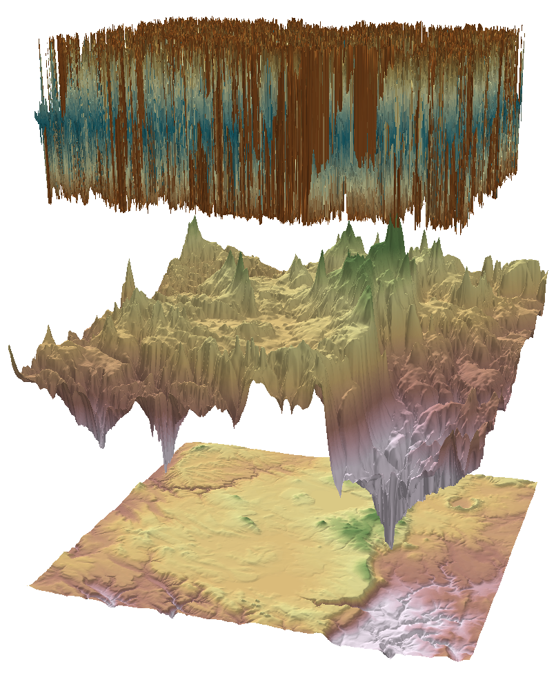
We are used to thinking of a flat sheet as two-dimensional and a solid block as three-dimensional. Mandelbrot (1967) pointed out that many natural shapes sit in between. His example was a coastline. Imagine measuring a stretch of coast by walking it with a measuring rod, swinging the rod end over end from one point on the shoreline to the next and counting the lengths. With a rod a hundred kilometers long you stride from headland to headland and never see the bays between them. With a ten-kilometer rod you have to go into every bay and out around every headland, and the coast comes out longer. With a one-meter rod you are picking your way around each boulder and tide pool, and it comes out longer still. It is the same coast every time; each shorter rod simply follows more of the detail that the longer one stepped across. (Mandelbrot pictured this being done on a map with a pair of dividers, the two-pointed compass a navigator steps across a chart, set to a smaller spacing on each pass.) From Richardson's measurements, as reported in Mandelbrot (1967), Mandelbrot put the west coast of Britain at D = 1.25. How fast the measured length grows as the rod gets shorter is the fractal dimension, somewhere between the 1 of a smooth curve and the 2 of a curve so wiggly it fills a plane. A landscape surface works the same way one dimension up. A perfectly smooth surface, flat or tilted, has a dimension of exactly 2; think of Nebraska. A surface so convoluted that it passes through every point in a volume would have a dimension of 3. Real terrain lies between, and the number tells you how much new detail appears each time you look more closely. Shelberg, Lam and Moellering (1983) report that “a fractal dimension of 2.3 is found to be a common value in describing the relief on the earth.”
This is why fractal dimension behaves differently from the Terrain Ruggedness Index or the surface ratio. Those measure how much the terrain departs from flat at one neighborhood size. Fractal dimension measures how that departure changes as you look more and more closely, at smaller and smaller pieces of the terrain. Two surfaces can have the same slope and the same local relief and still differ in D: one smoothly rolling, the other crinkly all the way down. And a smooth steep hillside scores exactly 2, the same as a plain, because tilting a plane does not give it any detail.
One quantity, four rulers
There is one important thing to understand before choosing a method. All four estimators here are trying to measure the same number, D, but each fits a scaling relationship in a different geometric or statistical domain, and real terrain is only approximately fractal: fractal over a limited range of scales, often different in different directions, and often more rough at some scales than others. So the estimators give different values on real DEMs. They do so even on ideal surfaces: all four rise and fall together as a surface gets rougher, but in development tests on artificial surfaces of known dimension, the variogram and madogram came closest to the true value, the prism method compressed high values (a surface with a true D of 2.75 came back as about 2.47, and lower still on surfaces with less relief, since this method responds to the size of the relief as well as its pattern), and box counting compressed them badly (true values from 2.15 to 2.75 came back as 1.92 to 2.16, raw values; this tool clips its output at 2, since no surface can have a dimension below 2). Ju and Lam (2009) put it plainly: “the problem of inconsistent results derived from different fractal calculation algorithms remains.” That is not a defect in any one method, and it is the opposite of the situation in the TRI tool, whose four methods are genuinely different quantities. The practical rule is simple: pick one estimator, stay with it throughout a study, and never compare a D value produced by one method with a D value produced by another.
Triangular prism (Clarke 1986; Ju and Lam 2009)
Clarke (1986) designed the triangular prism method for topographic surfaces, and it is a close relative of the Surface Area and Ratio tool. Lay a square of side S cells on the DEM, take the elevations at its four corners, interpolate a center elevation as their mean, and split the square into four three-dimensional triangles meeting at the center. Compute the area of those three-dimensional triangles with Heron's formula, exactly as the surface area tool does. (Each triangle, together with the column of ground beneath it, is a triangular prism, which is where the method gets its name.) Tile the whole window with squares of side S, build the four triangles on each square the same way, add up the areas of all those three-dimensional triangles, and call the total A(S). Now repeat with larger squares. A big square steps over small bumps on the landscape while a small square follows those bumps, so A(S) shrinks toward the flat footprint as S grows, and how fast it shrinks is the fractal dimension:
In the notation of calculus the same equation is written
The “d” stands for “a small change in”. The top of the fraction is a small change in log A, the bottom is the small change in log S that produced it, and one divided by the other is a rate of change: the slope of the curve of log A against log S. That is the normal way to write a slope in calculus, where it is called a derivative. It does not mean the dimension is worked out at a single step size. On a true fractal the curve is a straight line, with the same slope at every point; on real data the tool estimates that slope by fitting a line across all the step sizes, which is what the first form of the equation says in words. The other methods on this page are given in both forms too.
As with the other methods, one step size gives one area, and one area cannot give you a dimension. The tool computes A(S) for every step size, plots the logarithm of each area against the logarithm of its step size, and fits a straight line through the points; the slope of that line is what goes into the equation. The slope is negative, because the area shrinks as the squares grow, so subtracting it raises D above 2. Suppose a window on a 10 m DEM has a flat footprint of 57,600 m² and its total triangle area comes to 66,000 m² with 1-cell squares, 64,500 with 2-cell squares and 63,400 with 4-cell squares. The fitted slope of log area against log step is −0.029, so D = 2 + 0.029 = 2.03. A surface whose area did not shrink at all would have a slope of 0 and D = 2; a surface whose area halved every time the square doubled would have a slope of −1 and D = 3. The regression must be against log S, not log S² as Clarke's original used, which underestimated D; the corrected form is the one implemented here.
The squares do not overlap. This is an important point about the method, and an important difference from the variogram and madogram below. The quantity being measured is the total surface area of the window, and to measure an area you cover the ground exactly once, the way tiles cover a floor. So the squares sit edge to edge, each sharing its border cells with the next: in a 25-cell window, squares of side 8 cover cells 1 to 9, 9 to 17 and 17 to 25 in each direction, nine squares in all. There is no square covering cells 2 to 10 or 3 to 11. One consequence is that the large steps rest on very few squares:
| Step size in a 25-cell window | 1 | 2 | 3 | 4 | 6 | 8 | 12 |
|---|---|---|---|---|---|---|---|
| Squares tiling the window | 576 | 144 | 64 | 36 | 16 | 9 | 4 |
The point for a step of 12 on the log-log plot comes from just four squares, against 576 for a step of 1, and every point carries the same weight in the fitted line. The variogram and madogram work differently. At each lag they use every pair of cells the window holds, at every position, overlapping freely (1,200 pairs at a lag of 1 and still 850 at a lag of 8), because they are averaging a difference and have no area to cover. Differential box counting tiles its window differently. For each box size s it lays as many s-cell boxes as fit, floor(w/s) to a side, from the window's upper-left corner, with no shared border cells, using the sizes from the fixed series 2, 3, 4, 6, 8, 12, 16 and 24 cells that fit at least twice across the window. The boxes do not always cover the whole window: a 25-cell window is covered only by its upper-left 24 × 24 cells at every box size, and a 51-cell window by 48 to 51 cells depending on the size, so the box sizes are not compared over exactly the same ground in the way the prism steps are.
Because this is a moving window, the tiling moves with it. For one cell the squares of side 8 sit at cells 1 to 9, 9 to 17 and 17 to 25 of its window; for the cell next door the window has shifted by one cell, and so has every square in it. Over the whole raster, then, a square at every possible position does get measured, but each cell's D comes only from the squares that tile its own window. Two neighboring cells cover nearly the same ground and yet share none of their large squares: their values are computed from two different sets of squares laid over almost the same terrain.
That raises a fair question: would the method do better if each cell used the squares at every position in its window, overlapping, the way the variogram uses every pair? I tested the idea on artificial surfaces of known dimension, replacing the tiled total with the average area of a square at every position. It helped a little. The values were almost exactly the same as tiling gives (a correlation of 0.996 or higher), with somewhat less noise, most noticeably on the roughest surfaces in the smallest windows. But it did nothing for the method's real problem, which is bias and not noise. A surface with a true dimension of 2.5 came back as 2.01 to 2.09, depending on how much relief it had, and it came back as exactly the same numbers with overlapping squares as with tiled ones. So the tool follows the published method. The second consequence of tiling is that only certain step sizes will fit, which is the subject of the next paragraph.
For a moving window the step sizes have to be chosen with care, and Ju and Lam (2009) showed why: geometric steps of 1, 2, 4, 8 cells tile a window of arbitrary size poorly. The reason is that every step size has to cover the same ground, or the areas being compared are areas of different places. A square of side 8 spans 8 cell intervals, or 9 cells, and two of them side by side span 16 intervals, or 17 cells. So steps of 1, 2, 4 and 8 all tile a block of 17 cells exactly, and the next block they all tile exactly is 33 cells. A 29-cell window is too small to hold a 33-cell block, so only a 17 × 17 block of it can be used, which is 289 of its 841 cells, and the remaining two thirds are left out of the estimate. In the same way a 61 × 61 window holds a 33-cell block but not a 65-cell one, and in their table it uses only 29% of its cells. In general the doubling steps fit only windows of 2n + 1 cells (5, 9, 17, 33, 65), and any other size wastes whatever lies outside the largest such block. Their divisor-step method uses instead every step size that divides the window width minus one evenly, so that every step tiles the whole window with no leftover. For the default 25-cell window the steps are 1, 2, 3, 4, 6, 8 and 12 cells. You do not enter step sizes; the tool derives them from the window size you choose. Any odd window of 9 cells or more will run, but some sizes work better than others: the more divisors the width minus one has, the more steps go into the fit and the steadier it is. A 13-cell window gives steps of 1, 2, 3, 4 and 6; a 17-cell window gives 1, 2, 4 and 8; a 25-cell window gives the seven steps above; a 23-cell window gives only 1, 2 and 11. Sizes of 13, 25, 37, 49 and 61 all give five steps or more. The tool lists the steps it used in its run messages, and warns when only three fit, the fewest any window gives (9, 11, 15, 23, 27 and 35 cells, among others), naming 13, 17, 25, 33, 37, 49 or 61 as sizes that give four or more.
Variogram and madogram (Gneiting, Ševčíková and Percival 2012)
These two estimators come from spatial statistics rather than geometry, and they use the variation statistic of Gneiting, Ševčíková and Percival (2012), which is implemented in their R package fractaldim; the idea and the statistic are theirs, not mine. This tool departs from their implementation in two ways, described below. The question they ask is how the elevation difference between two cells grows with the distance between them. Take every pair of cells in the window that lie h cells apart along a row or a column, and average the absolute elevation difference raised to a power p. That separation h is called the lag, and the whole method turns on it, so it is worth being exact about what it means. At a lag of 1, every cell in the window is paired with its immediate neighbor along the row and with its immediate neighbor along the column. At a lag of 2, every cell is paired with the cell two over, skipping one. At a lag of 8, every cell is paired with the cell eight over. The tool pairs cells only along rows and columns, never diagonally. Each lag uses every such pair the window holds, so a 25-cell window supplies plenty of them, though fewer as the lag grows:
| Lag (cells) | 1 | 2 | 4 | 8 |
|---|---|---|---|---|
| Pairs along each row or column | 24 | 23 | 21 | 17 |
| Pairs in a 25 × 25 window | 1,200 | 1,150 | 1,050 | 850 |
Each lag boils all of its pairs down to a single number, the typical elevation difference between two cells that far apart:
With p = 2 this is the variogram (twice the semivariance familiar from kriging, since the mean here is not halved; the factor of two has no effect on D); with p = 1 it is the madogram, the mean absolute difference.
Vp(h) is one number for one lag h, and one number cannot give you a dimension. D comes from how Vp changes as h changes. So the tool computes Vp at every lag in its range (1, 2, 3 and so on), plots the logarithm of each against the logarithm of its lag, and fits a straight line through those points. On a fractal surface Vp grows as a power of the lag, and a power law is a straight line on logarithmic axes, which is why the logarithms are used. The slope of that fitted line is the measurement:
or, in calculus notation, where “d” means “a small change in” and the fraction is the slope of log Vp against log h:
A steep slope means the differences keep growing as the cells get farther apart, which is what a smooth surface does, and gives a D near 2. A shallow slope means neighboring cells already differ about as much as distant ones, which is what a rough surface does, and gives a D near 3. Dividing by p puts the variogram, which squares its differences and so doubles the slope, on the same footing as the madogram. (Gneiting et al. write this as D = 3 − α/2 and call α the fractal index; α/2 is the slope divided by p.)
Three madogram examples make the range concrete. On a smooth tilted plane the elevation difference between two cells is proportional to their separation, so if the mean absolute difference at lags of 1, 2, 4 and 8 cells is 1, 2, 4 and 8 m, the log-log slope is 1 and D = 3 − 1 = 2: a plane, as it should be. On a moderately rough surface the differences might be 1.00, 1.41, 2.00 and 2.83 m, growing by only the square root of 2 with each doubling of lag; the slope is 0.5 and D = 3 − 0.5 = 2.5. On pure noise, where every cell is unrelated to its neighbors, the difference is the same at every lag, 1, 1, 1 and 1; the slope is 0 and D = 3 − 0 = 3. A window with no variation at all is set to D = 2 directly, since a log of zero has no meaning.
So the recipe is: one typical difference per lag, plotted against the lag on logarithmic axes, a straight line fitted through the points, and D from the slope of that line. By default the tool uses lags from 1 cell up to a third of the window width (1 through 8 for the default 25-cell window), and it pools all the row and column pairs in the window into one average at each lag. Both of those differ from Gneiting et al.'s own implementation. They fit only lags 1 and 2, giving as their reason that the bias of the estimator grows as more lags are included, and for gridded data they compute a separate estimate along every row and every column and take the median of those. The Maximum lag parameter lets you choose the range yourself, and Which lags? below shows why the choice matters on a real DEM.
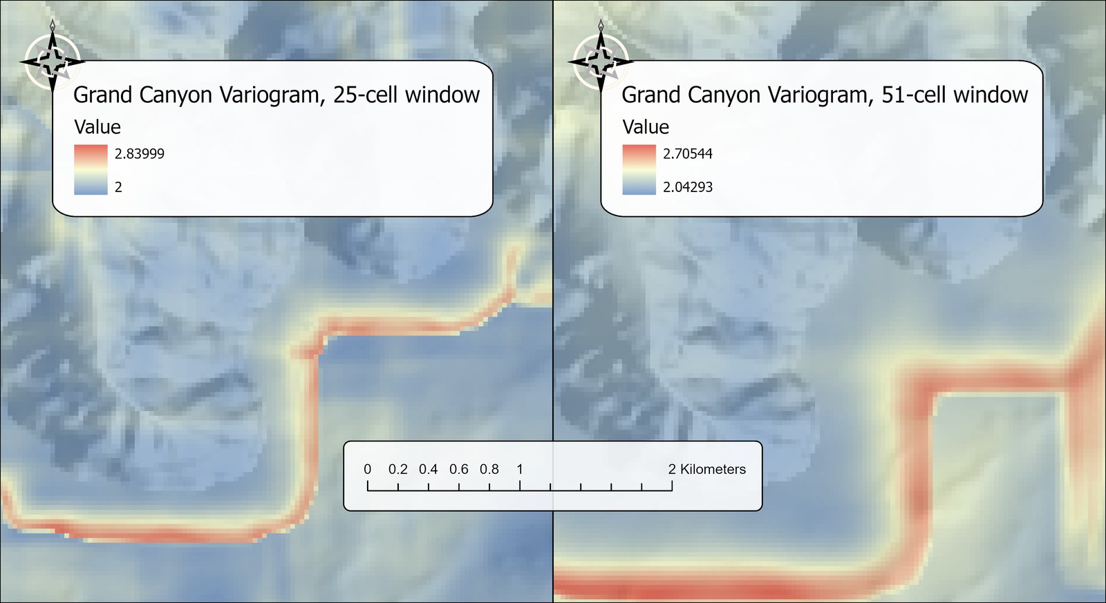
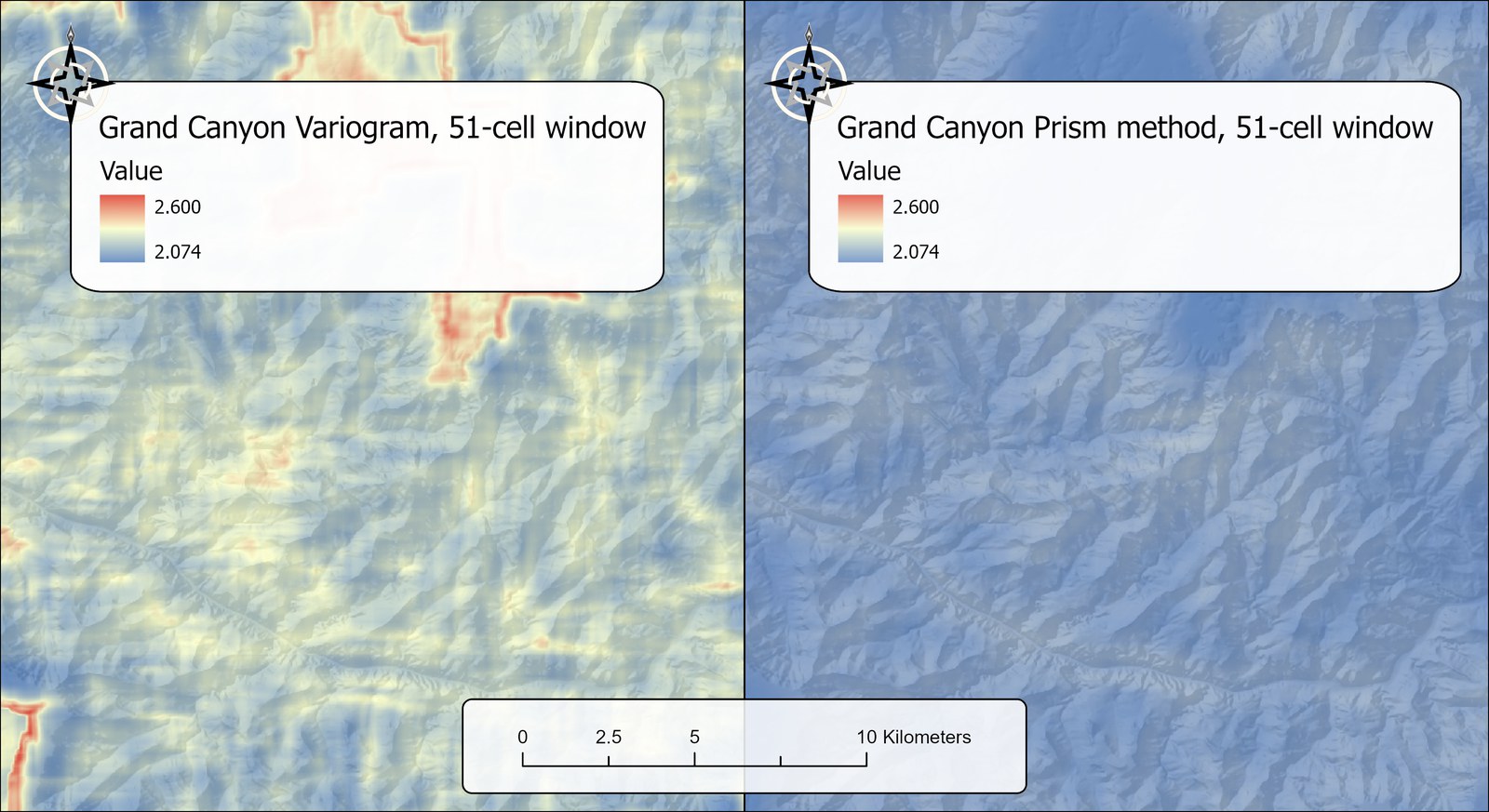
Two properties make these estimators strong recommendations as the default. In the simulations of Gneiting et al. the variogram had the lowest error on well-behaved data, the madogram was next, and box counting was last; they recommend the madogram because, considering both efficiency and robustness, it holds up better when the data are not well-behaved. And both are amplitude-invariant: multiply every elevation by ten, or express them in feet instead of meters, and Vp changes by a constant factor at every lag, which shifts the fitted line up without changing its slope. D does not depend on the vertical exaggeration at all, so these two methods reveal roughness on gentle terrain just as readily as on steep terrain. On a real Grand Canyon DEM the variogram gave the widest spread of values (about 2.04 to 2.71 with a 51-cell window), tracking the dissected tributary network against the plateaus, with the madogram a little smoother.
Which lags? A test on artificial surfaces and two real DEMs
If a surface follows a single power law, meaning that every time you double the distance between two cells the typical elevation difference multiplies by the same factor, whether you are going from a lag of 1 to a lag of 2 or from 8 to 16, then every lag tells the same story, the points fall on a straight line, and it hardly matters which lags go into the fit. On the moderately rough surface in the example above that factor is 1.41 at every doubling: 1.00, 1.41, 2.00 and 2.83 m.
The factor does not have to be any particular value, only the same value every time. A factor of 2 at every doubling is a plane, with a dimension of 2. A factor of 1.41 at every doubling is a dimension of 2.5. A factor of 1, meaning no growth at all, is a dimension of 3. So there are two separate questions to ask of the factors. How big are they? That gives the dimension. And are they all the same? That tells you whether the surface has a single dimension to give. A surface that follows a single power law has one value of D at every scale you examine it, and that one number describes its roughness completely. A surface whose factor changes from one doubling to the next has a D that depends on the lag distances you measure it over, and any one value you report belongs to that range of distances and no other. The two real DEMs below are of this second kind. (This is a statement about scale and not about place. Either kind of surface can still be rougher in one part of the raster than another, which is what the moving window maps.)
Two tests were run on the madogram and variogram to see how much the choice of lags matters in each case.
Artificial surfaces. The first test used computer-generated surfaces built to follow one power law exactly, with a known fractal dimension (2.1, 2.3, 2.5, 2.7 and 2.9), and about 12,000 windows on each. Here there is a right answer, and two lags came closer to it. The typical error of the madogram in a 25-cell window was 0.048 with lags 1 and 2 against 0.069 with lags 1 through 8, and in a 51-cell window 0.029 against 0.062. This agrees with Gneiting et al.: on a surface that really is a fractal, the long lags add bias and noise and the short lags carry the information.
Real DEMs. The second test used two real DEMs: the 1-arc-second Grand Canyon DEM in the examples on this page, and the 30 m DEM from the Corridor Designer tutorial data, gentler country whose elevations are stored as whole meters. A real DEM has no known dimension to compare with, so the test asks something else: does the DEM follow a single power law at all? The test is the one described above: does the typical difference multiply by the same factor at every doubling of the lag? The table takes it one step at a time. The first row for each DEM is the typical elevation difference (the madogram's mean absolute difference) over the whole DEM at lags of 1, 2, 4, 8 and 16 cells. The second row is each value divided by the one before it, which is the factor for that doubling: 19.9 ÷ 10.4 ≈ 1.9, and so on. The third row turns each factor into the fractal dimension it implies. The factors, dimensions and multiples in these tables were computed from the unrounded differences, so recomputing them from the rounded values shown can differ in the last digit. Doubling the lag moves one step of log 2 along the horizontal axis of the log-log plot, so the slope between the two points is the base-2 logarithm of the factor, and D = 3 − log2(factor): 3 − log2(1.92) = 3 − 0.94 = 2.06.
| Lag (cells) | 1 | 2 | 4 | 8 | 16 |
|---|---|---|---|---|---|
| Grand Canyon: typical difference | 10.4 m | 19.9 m | 36.9 m | 65.3 m | 108 m |
| factor from the lag before | 1.92 | 1.86 | 1.77 | 1.66 | |
| D implied by that factor | 2.06 | 2.11 | 2.17 | 2.27 | |
| Gentler 30 m DEM: typical difference | 3.1 m | 5.9 m | 10.5 m | 17.0 m | 26.1 m |
| factor from the lag before | 1.90 | 1.76 | 1.62 | 1.53 | |
| D implied by that factor | 2.08 | 2.18 | 2.30 | 2.38 | |
| A true fractal with D = 2.5, for comparison: factor | 1.41 | 1.41 | 1.41 | 1.41 |
Neither DEM is a single power law. The factor falls steadily on both, where a single power law would hold it constant, and so the implied dimension climbs from one doubling to the next. Both DEMs read almost perfectly smooth at the shortest lags, with a dimension barely above 2, and rougher as the distance grows. On the log-log plot the points make a curve, steep at the left and flatter to the right, and a straight line fitted to a curve has a slope that depends on which part of the curve you fit. The variogram shows the same pattern.
The gentler DEM reads a higher dimension than the Grand Canyon at every doubling, which may come as a surprise, and the reason is worth understanding. Fractal dimension measures how fast the elevation differences grow with distance, not how large they are. Look again at the typical differences in the table above, this time with each one expressed as a multiple of its own DEM's value at a lag of 1:
| Typical difference as a multiple of the lag-1 value, at a lag of… | 1 cell | 2 cells | 4 cells | 8 cells | 16 cells |
|---|---|---|---|---|---|
| Grand Canyon (10.4 m at lag 1) | 1 | 1.9 | 3.6 | 6.3 | 10.5 |
| Gentler 30 m DEM (3.1 m at lag 1) | 1 | 1.9 | 3.4 | 5.4 | 8.3 |
| A smooth tilted plane, for comparison | 1 | 2 | 4 | 8 | 16 |
The Grand Canyon's differences are three to four times larger at every lag, which is the ruggedness everyone sees. But they also keep growing with distance, closer to the way a plane's do: 16 cells apart, they are 10.5 times the lag-1 value, against 8.3 times on the gentler DEM. That is what long continuous slopes produce, since on a canyon wall going twice as far means dropping nearly twice as much. On the gentler DEM the differences accumulate more slowly, which is what smaller landforms produce: when a lag is long enough to carry you over a rise and part of the way down the other side, the two ends stop growing more different. Slower growth is a higher D. So a high fractal dimension does not mean big relief. It means relief organized into features that are small compared with the lags being measured. This is the sense in which fractal dimension, like VRM, is independent of slope, and it is why it should be read alongside a measure of relief and not in place of one.
Two things could make a DEM read smooth at a lag of one or two cells, and this test cannot tell them apart. The ground may really be smooth over 30 to 60 m. And a DEM is an interpolated product, so neighboring cells may share some of the same source measurements. Either way, a lag of one 30 m cell is a long way from the vanishingly small distance at which fractal dimension is defined.
The practical consequences show up in the output rasters. The numbers below are for the madogram:
| Lags 1 and 2 | Default lags (one third of the window) | |
|---|---|---|
| Grand Canyon, 25-cell window: mean D (standard deviation) | 2.06 (0.03) | 2.13 (0.07) |
| Grand Canyon, 51-cell window | 2.06 (0.02) | 2.19 (0.08) |
| Gentler DEM, 25-cell window | 2.07 (0.05) | 2.18 (0.11) |
| Gentler DEM, 51-cell window | 2.07 (0.04) | 2.25 (0.12) |
- The two choices make different maps. The correlation between the two-lag raster and the default raster in the Grand Canyon was 0.76 with a 25-cell window and 0.54 with a 51-cell window. They are measuring roughness at different scales: one or two cells in the first case, and everything out to a third of the window in the second.
- Two lags give a low-contrast map. Nearly every value falls in a narrow band just above 2, because at that scale nearly all of the terrain reads smooth.
- Whole-number elevations disturb the shortest lags a little, on gentle ground only. Rounding the floating-point Grand Canyon DEM to whole meters and running it again changed almost nothing overall. The effect was confined to the gentlest windows, those where neighboring cells differ by less than half a meter, and it was larger for two lags than for the default: the share of those windows falling below the valid minimum of 2 (and clipped to 2) rose from 5.8% to 9.8% with two lags, and from 5.5% to 5.9% with the default lags.
- The default range grows with the window. A 25-cell window fits lags 1 through 8 and a 51-cell window fits 1 through 17, so with the default, changing the window changes both the area summarized and the scales measured. That is why the mean rises from 2.13 to 2.19 in the Grand Canyon. With the maximum lag fixed at 2 the mean stays at 2.06 for both windows.
Projected DEMs. Because the lags run along rows and columns, it is fair to ask what a projected DEM does to them, since projecting a raster means resampling it. A third test resampled the Grand Canyon DEM onto a slightly rotated and rescaled grid by nearest neighbor, bilinear interpolation and cubic convolution, and ran the madogram and variogram on each (25-cell window, default lags):
| Mean D | Original grid | Nearest neighbor | Bilinear | Cubic convolution |
|---|---|---|---|---|
| Madogram | 2.130 | 2.139 | 2.117 | 2.130 |
| Variogram | 2.193 | 2.203 | 2.163 | 2.186 |
The repeats and skips of nearest neighbor, which do so much damage to slope, matter little here. Slope is built from a handful of neighbors, so one repeated cell shows; each lag in this tool averages about a thousand pairs, and a repeat (a difference of zero) and a skip (a double-sized difference) largely cancel in that average. The larger effect is from bilinear interpolation, which averages neighboring cells and so smooths the surface at exactly the shortest lags: it lowered the mean D by 0.013 for the madogram and 0.030 for the variogram, and by 0.017 and 0.047 when only lags 1 and 2 were used. Cubic convolution stayed closest to the original. These are small shifts next to the differences between methods and between lag ranges above, but they are systematic, so compare fractal dimension rasters only when they come from DEMs prepared the same way. The cleanest choice is to run the tool on the DEM in its original coordinate system; it accepts geographic DEMs directly.
The default stays at one third of the window, because on these two DEMs it gave the map with more contrast and was less sensitive to rounded elevations. Enter a Maximum lag when you have a reason to: 2 to follow Gneiting et al. exactly, or any fixed value when you want to compare window sizes over the same range of distances. Whichever you use, the lags are listed in the run messages and recorded in the output raster's metadata, and the dimension you report should be described as the dimension over that range of distances (30 to 240 m, for lags 1 through 8 on a 30 m DEM) and not as a single property of the landscape.
Differential box counting (Sarkar and Chaudhuri 1994)
Box counting follows most directly from the definition of fractal dimension, and differential box counting is a well-established method for images (Nayak et al. 2019). Important: I include this method mainly because it is commonly discussed in the literature, not because I think it is the best estimator. See below for a discussion of the quality of the estimates. Divide the window into tiles of s × s cells. Over each tile, stack cubes s cells on a side (in true ground units, so a cube on a 10 m DEM with s = 2 is 20 m tall) and count how many are needed to span the tile's elevation range from its lowest cell to its highest: the range divided by the cube height, rounded up, or 1 if the tile is flat. Add the counts over all the tiles to get N(s), repeat for a series of tile sizes, and
or, in calculus notation, where “d” means “a small change in” and the fraction is the slope of log N against log s:
Here too the dimension comes from a fitted line and not from any one tile size: the tool plots the logarithm of each count against the logarithm of its tile size and fits a straight line through the points. The counts fall as the tiles grow, so the slope is negative, and D is that slope with its sign reversed. On a flat or smoothly tilted window every tile needs one box, so with a 25-cell window and tile sizes of 2, 3, 4, 6, 8 and 12 the counts are 144, 64, 36, 16, 9 and 4: the number of tiles. The log-log slope is exactly −2 and D = 2. On rough terrain the small tiles need extra boxes to span their relief, so the counts might be 300, 120, 62, 25, 13 and 5; the slope is −2.28 and D = 2.28. The box is a true cube in ground units, and the count for a tile is its elevation range divided by the box height, rounded up, counted from the tile's own lowest cell rather than from a fixed zero. That counting rule is the second of three refinements proposed by Li, Du and Sun (2009), who showed that the original method can count more boxes than a tile needs. The tool does not use their other two refinements (a reduced box height tied to the image's standard deviation, and overlapping tiles), which were designed for gray-level images rather than for terrain in real ground units. The tool starts the tile sizes at 2 rather than 1, because a single-cell tile has no elevation range and would anchor the regression at a meaningless point.
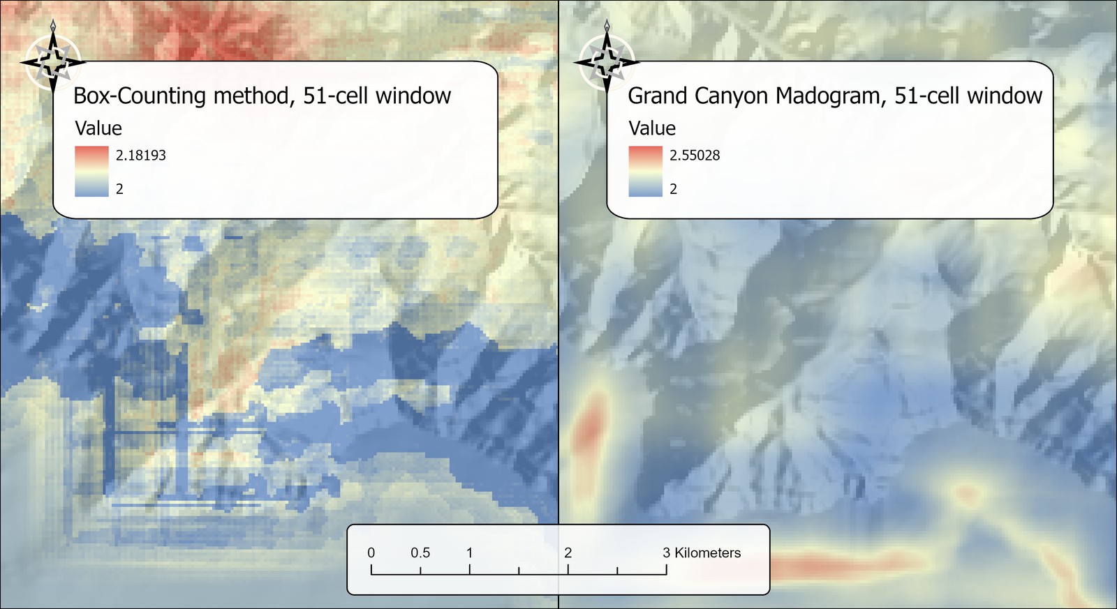
A word of warning: This box counting method, using a moving window approach, is the weakest and noisiest of the four methods for estimating fractal dimension. Only a handful of tile sizes fit a window (six for a 25-cell window), the counts are coarse whole numbers, and so the fitted slope wobbles. Gneiting et al. (2012) rank box counting the least efficient of the estimators they studied. In practice this gives it a compressed range, separating smooth from rough terrain less sharply than the other methods (about 2.00 to 2.18 on the same Grand Canyon DEM where the variogram spanned 2.04 to 2.71), and its raw slope can occasionally imply a value slightly under 2. A surface cannot truly have a fractal dimension below 2, so the tool clips every method's output to the range 2 to 3. It also has a visual artifact of its own, described below. Prefer the triangular prism or, especially, the variogram or madogram when you need the most reliable local estimate.
Vertical and horizontal units
The triangular prism and box-counting methods measure the terrain's actual three-dimensional shape, so elevation must be in the same unit as horizontal distance: true one-to-one ground units, with no vertical exaggeration and no per-window normalization. If the DEM's elevations are in feet on a coordinate system in meters, set Elevation units to feet and the tool converts internally. The tool reads the units from the DEM's vertical coordinate system and locks the setting when it can, assumes meters for geographic DEMs, and asks you only when the DEM does not say. One consequence of true one-to-one units is worth knowing: gently rolling terrain, whose relief is small compared with its cell size, genuinely is close to a plane, so these two methods read it near D = 2 and only steep, broken terrain drives them toward 3. In a test raster with 10 m cells and 20 to 30 m of relief the prism method stayed between about 2.05 and 2.11 while the variogram spanned 2.13 to 2.48. The variogram and madogram, being amplitude-invariant, are unaffected by this setting and by the steepness of the terrain, which is one more reason to prefer them as the default.
The prism and box-counting methods use one cell size for the whole DEM, the mean of the cell's east–west and north–south dimensions: on a projected DEM the mean of the two cell dimensions, and on a geographic DEM the mean of the two ground dimensions at the DEM's central latitude. The Grand Canyon DEM's cells, about 25 m east–west by 31 m north–south, are therefore treated as 28 m squares. Because fractal dimension is a scale analysis and the cell size varies only slightly across any one window, this approximation is immaterial to the result.
The window, and two artifacts to recognize
The window is a square of the odd width you choose, at least 9 cells, centered on each cell; the default is 25. A larger window gives a more stable estimate, because more pairs and more step sizes go into each regression, but a coarser and more smoothed result and a wider blank border. A window must be entirely free of NoData to produce a value, so every cell within half a window of the raster edge or of any NoData gap is NoData in the output.
The edge halo. Because D is estimated within a window, results near an abrupt boundary between two different kinds of terrain, such as the flat rim and the steep wall of a canyon, a cliff, or an escarpment, can show a ring of high (or low) values about half a window out from the boundary. There the window straddles both terrains and is fitting one dimension to a mixed surface that no single D describes, so the estimate is unreliable. I first saw this on a Grand Canyon DEM, where the variogram peaked about 700 m out from the rim on the smooth plateau side, half of the 51-cell window I had used, and I wondered whether the transition zone was intrinsically the most fractal terrain. It is not. On a synthetic plateau, wall and floor with no real roughness anywhere, the same halos appear at about half a window on either side of the wall, and they move outward when the window grows. That is the diagnostic: if a band of extreme values sits about half a window from a sharp edge and moves when you change the window size, it is the window, not the terrain. (A clean, steep wall on its own tends to read low, near 2, because a single dominant step is locally smooth in the fractal sense; the high values are beside it, not on it.) The same caution applies within half a window of the raster edge or of any NoData gap. Smaller windows shrink the ring but give a noisier estimate, which is a genuine trade-off.
The box-counting moiré. Differential box counting alone can show a blocky, repeating texture at roughly a half and a third of the window width. The cause is the largest tile sizes: for a 51-cell window the two largest are 24 and 16 cells, which divide the window into only two and three whole tiles, and those few coarse, grid-aligned, whole-number counts dominate the regression and stamp their pattern into the result at the scale of the tiles. The triangular prism and variation methods do not do this, which is another reason to prefer them.
A tour of the dialog
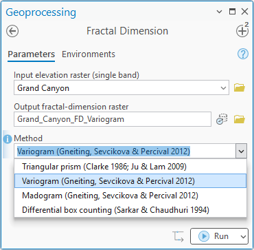
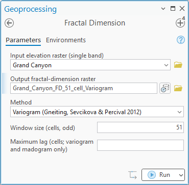
The dialog asks for the DEM, an output name, the estimator, the window size in cells, the DEM's elevation units and, for the variogram and madogram only, an optional maximum lag. The window size is a single odd number; the tool derives the step sizes, lags or tile sizes from it. For the triangular prism method a size whose width minus one has many divisors, such as 13, 25, 37, 49 or 61, gives more steps and a steadier fit. The output is a floating-point raster clipped to the range 2 to 3, with statistics, a histogram and bilinear pyramids already built, so it draws correctly the moment it reaches the map, with a blue-yellow-red stretch applied by default.
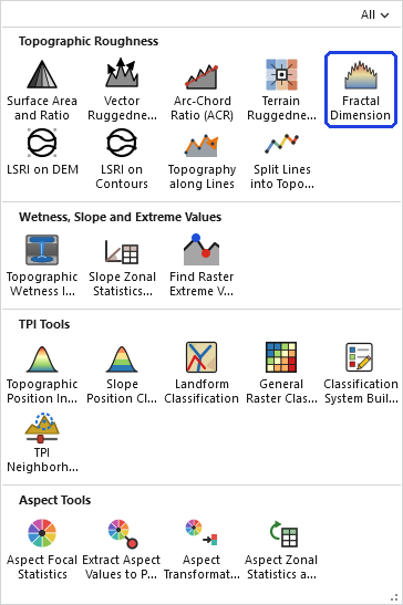
The tool holds the whole DEM in memory at once, so the memory it needs grows with the number of cells. On most DEMs that is no concern. On a very large one the tool may need more memory than your computer has free, and then one of two things happens: Windows starts using the disk as overflow memory and the tool slows to a crawl, or the tool stops with an out-of-memory error. There is no fixed limit; it depends on how much memory your computer has free. If a DEM is too large, clip it to the area you need first.
ModelBuilder
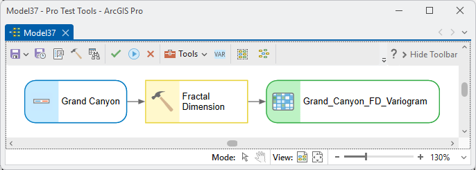
Parameters
| Label | Explanation | Data type |
|---|---|---|
| Input elevation raster (single band)Required · in_raster | The DEM. Must be single band; projected or geographic (a geographic DEM uses a representative ground cell size at its central latitude). | Raster Layer |
| Output fractal-dimension rasterRequired · out_raster | The local fractal dimension D of each cell's window, floating point, clipped to 2 (smooth) through 3 (maximally rough). NoData wherever the window is not entirely within valid data. A name is suggested from the input. A folder output without an extension becomes a GeoTIFF. | Raster Dataset |
| MethodRequired · method | Triangular prism (Clarke 1986; Ju & Lam 2009), Variogram (Gneiting, Sevcikova & Percival 2012), Madogram (Gneiting, Sevcikova & Percival 2012) or Differential box counting (Sarkar & Chaudhuri 1994). All estimate the same D; pick one and stay with it. The variogram or madogram is the recommended default; the dialog opens on Variogram, and the method, window size and elevation units are remembered from the last run. | String |
| Window size (cells, odd)Required · window_size | Side of the square moving window in cells; odd and at least 9; default 25. Larger windows give a more stable but coarser estimate and a wider NoData border. For the triangular prism method a size whose width minus one has many divisors (13, 25, 37, 49 or 61) gives more steps and a steadier fit. Every method accepts any odd size of 9 or more. | Long |
| Elevation unitsOptional · elev_units | Meters or Feet. Filled in and locked from the DEM's vertical coordinate system when it has one; geographic DEMs are assumed to be in meters; you are asked only when the DEM does not say. Affects the triangular prism and box-counting methods, which need true one-to-one units; the variogram and madogram are amplitude-invariant and unaffected. | String |
| Maximum lag (cells; variogram and madogram only)Optional · max_lag | The longest lag used by the variogram and madogram methods, between 2 and half the window size. Leave it blank for lags 1 through one third of the window (1 through 8 for a 25-cell window). Enter 2 for the two lags of Gneiting et al. (2012). See Which lags? Unavailable for the triangular prism and box-counting methods, which derive their own step and box sizes from the window. Unlike the other settings, it is not remembered between runs. | Long |
Python
import arcpy
arcpy.ImportToolbox(r"C:\path\to\JennessEnterprisesTools.pyt")  # your install path
# The recommended madogram estimator with the default 25-cell window.
arcpy.jenness.FractalDimension(
    in_raster=r"C:\Project\Elev.gdb\DEM",
    out_raster=r"C:\Project\Elev.gdb\DEM_FD_madogram",
    method="Madogram (Gneiting, Sevcikova & Percival 2012)",
    window_size=25, elev_units="Meters")
# The same, fitted to lags 1 and 2 only, as in Gneiting et al. (2012).
arcpy.jenness.FractalDimension(
    in_raster=r"C:\Project\Elev.gdb\DEM",
    out_raster=r"C:\Project\Elev.gdb\DEM_FD_madogram_lag2",
    method="Madogram (Gneiting, Sevcikova & Percival 2012)",
    window_size=25, elev_units="Meters", max_lag=2)
# The triangular prism method for comparison (window 25: steps 1,2,3,4,6,8,12).
arcpy.jenness.FractalDimension(
    in_raster=r"C:\Project\Elev.gdb\DEM",
    out_raster=r"C:\Project\Elev.gdb\DEM_FD_prism",
    method="Triangular prism (Clarke 1986; Ju & Lam 2009)",
    window_size=25, elev_units="Meters")
# Other method strings: "Variogram (Gneiting, Sevcikova & Percival 2012)",
# "Differential box counting (Sarkar & Chaudhuri 1994)".
Recommended citation
Credits and references
By Jeff Jenness, Jenness Enterprises (www.jennessent.com). The variogram and madogram estimators are a reimplementation of the variation estimator of Gneiting, Ševčíková and Percival (2012) and their R package fractaldim; the triangular prism method follows Clarke (1986) as adapted to a moving window by Ju and Lam (2009); differential box counting follows Sarkar and Chaudhuri (1994), with the box-counting rule of Li, Du and Sun (2009) and boxes that are true cubes in ground units. Sun et al. (2006) and Nayak et al. (2019) review the family of methods, and Shelberg, Lam and Moellering (1983) is an early treatment of surface fractal dimensions in cartography.
- Clarke, K. C. 1986. Computation of the fractal dimension of topographic surfaces using the triangular prism surface area method. Computers & Geosciences 12:713–722. doi.org/10.1016/0098-3004(86)90047-6
- Gneiting, T., H. Ševčíková, and D. B. Percival. 2012. Estimators of fractal dimension: assessing the roughness of time series and spatial data. Statistical Science 27:247–277. doi.org/10.1214/11-STS370. R package fractaldim: CRAN.R-project.org/package=fractaldim
- Jenness, J. Topographic roughness. Lecture, GIS for wildlife and forestry courses, Jenness Enterprises. Slides
- Ju, W., and N. S.-N. Lam. 2009. An improved algorithm for computing local fractal dimension using the triangular prism method. Computers & Geosciences 35:1224–1233. doi.org/10.1016/j.cageo.2008.09.008
- Li, J., Q. Du, and C. Sun. 2009. An improved box-counting method for image fractal dimension estimation. Pattern Recognition 42:2460–2469. doi.org/10.1016/j.patcog.2009.03.001
- Mandelbrot, B. B. 1967. How long is the coast of Britain? Statistical self-similarity and fractional dimension. Science 156:636–638. doi.org/10.1126/science.156.3775.636
- Nayak, S. R., J. Mishra, and G. Palai. 2019. Analysing roughness of surface through fractal dimension: a review. Image and Vision Computing 89:21–34. doi.org/10.1016/j.imavis.2019.06.015
- Sarkar, N., and B. B. Chaudhuri. 1994. An efficient differential box-counting approach to compute fractal dimension of image. IEEE Transactions on Systems, Man, and Cybernetics 24:115–120. doi.org/10.1109/21.259692
- Shelberg, M. C., N. Lam, and H. Moellering. 1983. Measuring the fractal dimensions of surfaces. Proceedings, Sixth International Symposium on Automated Cartography (Auto-Carto 6). Defense Technical Information Center report ADA129664. doi.org/10.21236/ADA129664
- Sun, W., G. Xu, P. Gong, and S. Liang. 2006. Fractal analysis of remotely sensed images: a review of methods and applications. International Journal of Remote Sensing 27:4963–4990. doi.org/10.1080/01431160600676695
Licensing information
Works at every ArcGIS Pro license level (Basic, Standard, Advanced). No extension licenses are required; the estimators are computed internally, without Spatial Analyst.
Related tools and pages
- About Topographic Roughness — choosing among the nine roughness measures.
- Vector Ruggedness Measure (VRM) — the other slope-independent index, measured at one neighborhood size.
- Surface Area and Ratio — the triangle areas the prism method is built from.
- Terrain Ruggedness Index (TRI) — single-scale roughness, whose four methods are different quantities rather than different estimators of one.
- Topography along Lines — the fractal dimension of a route, by the divider method, as a line attribute.
- Projecting Rasters — this tool works on geographic DEMs directly; if you project a DEM first, use cubic convolution, which in the resampling test above stayed closest to the original, while bilinear interpolation lowered D the most.