

LSRI on Contours
Summary
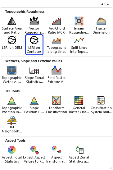
Computes the Land Surface Ruggedness Index (LSRI) of Beasom, Wiggers and Giardino (1983) from contour lines you already have: the total length of polyline within a circular neighborhood of every cell of a new raster. Sappington et al. (2007) called LSRI the first widely recognized method for quantifying ruggedness among biologists. The input is any polyline feature class, typically elevation contours but also roads, streams or trails, and if the input has a selection only the selected features are measured. You choose the output cell size, the neighborhood radius and the length units. Correct on geographic (latitude/longitude) data, with no Spatial Analyst or 3D Analyst license needed. The companion LSRI on DEM tool traces the contours from a DEM for you and carries the full explanation of the index; this page covers what is different when you start from lines.
When to start from lines instead of a DEM
Beasom et al. (1983) worked from printed topographic maps, and the quantity behind their index was the total length of contour line inside a 40-hectare circle; the LSRI on DEM page tells that story and explains why contour length is a sensible measure of ruggedness, how the contour interval scales the values, and how the tool measures length inside a circle exactly. Everything there applies here. The difference is only where the lines come from. There are three good reasons to supply them yourself:
- You already have contours. Published contour data, contours from a survey, or the contour feature class that LSRI on DEM saved on an earlier run, when you want to try another radius without contouring the DEM again. Any contour lines work, at any interval; just remember that the interval sets the magnitude of the values, so keep it the same across the runs you compare.
- You want to measure a subset. Because the input is a feature layer, an active selection is honored automatically, the standard ArcGIS Pro behavior for that kind of input. Select only the contours above tree line, or only the index contours, and the tool measures those alone.
- The lines are not contours at all. The tool measures the total length of whatever polylines you give it within each circle. Run it on a stream network and you have the length of channel around every cell, which is the raw material of drainage density, the length of channel per unit area that Melton (1957), as described by Beasom et al. (1983), multiplied by total relief to get his ruggedness number for drainage basins. Run it on roads, trails or fence lines and you have the length of those around every cell. Keep in mind that what comes out is a total length and not a density; if it is a density you want, see the next paragraph.
Whatever the lines are, the tool reports the total length inside the circle, in the units you choose. That is the quantity Beasom et al. measured. If you want a density, use Esri's Line Density tool, which reports length per unit area directly and is built for that purpose. (You could also divide this tool's output by the area of the circle, πr², in matching units: a 500 m radius covers 0.785 km², so 3,140 m of line inside the circle would be 4.0 km per km². But that is Line Density's job, and this tool does not call it.)
What the tool does
The tool reads the polylines (only the selected ones, if there is a selection), breaks every line into its straight segments, and creates a new raster of the cell size you choose covering the input's extent, expanded outward by the radius (or, if the Extent geoprocessing environment is set, exactly that extent, with no expansion). The expansion lets cells just outside the data still see the lines that fall within their circles; it is not an edge correction. A cell whose circle reaches beyond the data has less line available to it than an interior cell, so values within one radius of the data's edge, and in the added ring, run low and should be read as edge artifacts. Then, for every cell, it adds up the exact length of line inside the circle of the chosen radius around the cell center, using the same closed-form segment-and-circle clip described on the LSRI on DEM page. To take the same example, a 300 m segment that runs from 100 m west of a cell center to 200 m east of it, passing 100 m to the north, contributes 273.2 m to that cell at a 200 m radius: the part inside the circle, from −100 m to +173.2 m, and not a meter more.
On a geographic (latitude/longitude) feature class, the vertices and cell centers are converted to Earth-centered coordinates in meters on the data's reference spheroid before the clip, so the neighborhood is a true ground circle and the lengths are true ground lengths at any latitude. A ground-unit radius (meters, kilometers, feet, miles) needs no approximation at all; the Cells unit uses one representative ground cell size at the data's central latitude. Projected data are measured directly in their own map units.
Cell size
Because there is no DEM to inherit a grid from, you set the output cell size yourself, in the input's map units. The default is the greater of the input extent's width or height divided by 1,000, which puts about a thousand cells across the longer side of the data: for a feature class 24 km wide and 18 km tall the default is 24 m. That default is meant to give a reasonably detailed raster without an unreasonable run time, and it is only a starting point. A finer cell size gives a smoother, more detailed surface at the cost of proportionally more cells to evaluate (halving the cell size quadruples the count); a coarser one is faster and may be all a habitat model needs. The cell size does not change the values themselves, only where they are sampled, since each value is the length inside a circle of the same radius regardless of the grid.
Radius
As with LSRI on DEM there is no default radius the first time; after that the dialog pre-fills the last run's radius and units, and the units start at Meters. Beasom et al.'s 40 ha circle is about 356.8 m if you want to reproduce their scale. Beasom et al. do not say why they chose 40 hectares; it may have just been a practical size to trace by hand on a printed 7.5-minute map, and a computed neighborhood need not honor it. Choose the scale of your question, try two or three radii, and compare runs only at the same radius and the same contour interval, since both change the magnitude of every value.
A tour of the dialog
The example continues from the LSRI on DEM page: the 10 m contours that tool saved from the Grand Canyon DEM are the input here, and the question is what LSRI looks like when only every fifth contour, the 50 m intervals, are measured.
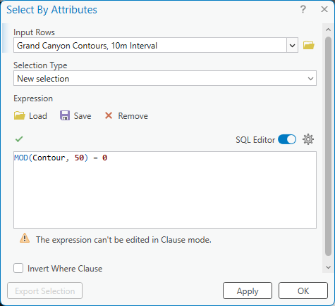
MOD(Contour, 50) = 0 keeps every
contour whose elevation is a multiple of 50. It is not the
only way to make this selection, but it works with the
contour feature classes these tools generate, because they
write each contour's elevation to a field named
Contour at an exact multiple of the interval. (If you
contoured from a base other than 0, subtract the base first:
MOD(Contour - 5, 50) = 0. Shapefiles do not
support MOD; list the elevations with IN instead.)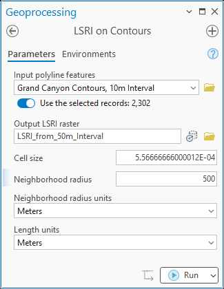
The dialog asks for the polyline layer or feature class, the output raster name, the cell size (filled in from the extent until you change it), the radius and its units, and the length units of the output values. If the input layer has a selection, Pro notes the number of selected records beneath the input in the tool dialog, and only those features are used.
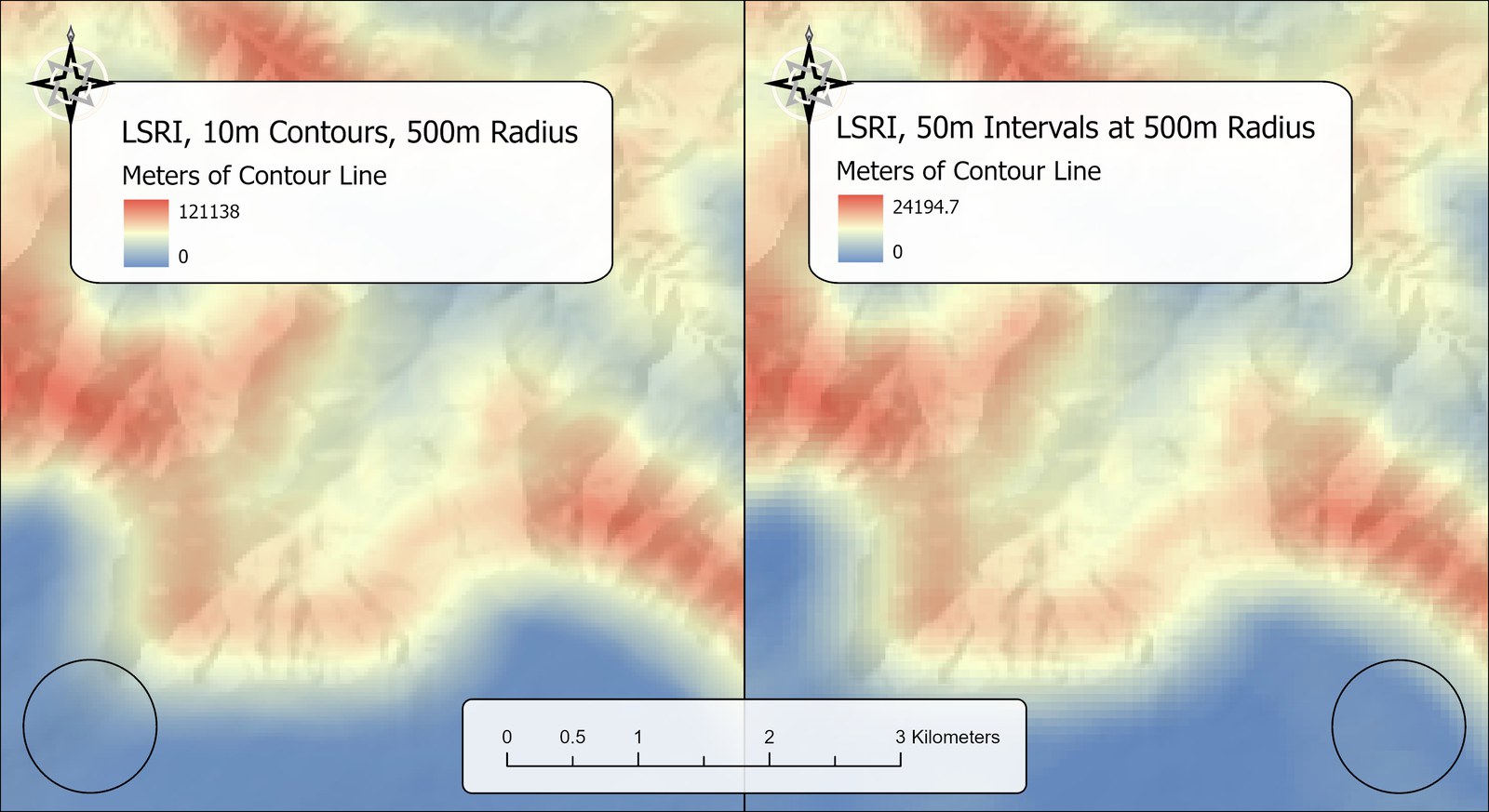
The output is a floating-point raster of lengths in the chosen units, 0 where no line falls within the circle and climbing from there without an upper bound. It carries statistics, a histogram and pyramids and draws with the same blue-yellow-red stretch as the other roughness tools. A folder output without an extension becomes a GeoTIFF.
A run stops with an error above 5,000,000 input segments, or 20,000,000 of the pieces they are subdivided into. The piece limit is the one long lines can reach, such as roads or transmission lines with a small radius; the remedies are fewer or simpler lines, a smaller extent, or a larger radius.
ModelBuilder
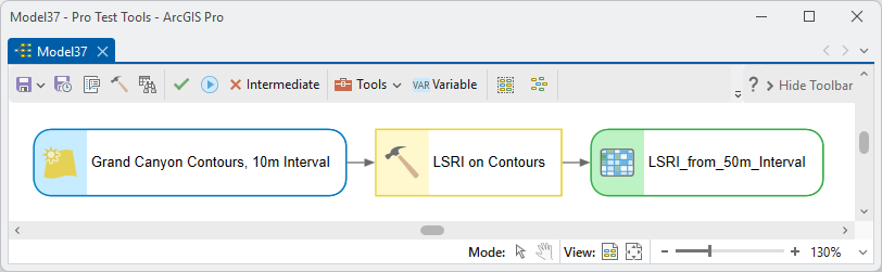
Parameters
| Label | Explanation | Data type |
|---|---|---|
| Input polyline featuresRequired · in_polylines | The polylines to measure: typically elevation contours, but any polyline data. Projected or geographic. If the input has an active selection, only the selected features are used. | Feature Layer |
| Output LSRI rasterRequired · out_raster | The total length of polyline within the neighborhood radius of each cell, in the length units. Floating point. A name is suggested from the input. | Raster Dataset |
| Cell sizeRequired · cell_size | The output raster's cell size in the input's map units. Defaults to the greater of the input extent's width or height divided by 1,000. | Double |
| Neighborhood radiusRequired · radius | How far the circle extends around each cell, in the radius units. No default: choose the scale that suits your question (Beasom et al.'s 40 ha circle is about 356.8 m). Larger radii give larger values. | Double |
| Neighborhood radius unitsRequired · radius_units | Cells (that many output cells, using the cell size above), Meters, Kilometers, Feet or Miles (converted to the input's map units; exact on geographic data). | String |
| Length unitsOptional · length_units | The units of the output values: Meters (default), Feet, Kilometers or Miles. | String |
Python
import arcpy
arcpy.ImportToolbox(r"C:\path\to\JennessEnterprisesTools.pyt")  # your install path
# LSRI from an existing contour feature class, 30 m cells, 500 m neighborhood.
arcpy.jenness.LSRIOnContourPolylines(
    in_polylines=r"C:\Project\Elev.gdb\DEM_Contours",
    out_raster=r"C:\Project\Elev.gdb\Contours_LSRI",
    cell_size=30, radius=500, radius_units="Meters",
    length_units="Meters")
# The same tool on a stream network: total channel length within 1 km of each cell.
arcpy.jenness.LSRIOnContourPolylines(
    in_polylines=r"C:\Project\Hydro.gdb\Streams",
    out_raster=r"C:\Project\Hydro.gdb\Stream_Length_1km",
    cell_size=50, radius=1, radius_units="Kilometers",
    length_units="Kilometers")
Recommended citation
Credits and references
By Jeff Jenness, Jenness Enterprises (www.jennessent.com), automating the contour-length measurement of Beasom, Wiggers and Giardino (1983) over a moving neighborhood, from polylines supplied by the user.
- Beasom, S. L., E. P. Wiggers, and J. R. Giardino. 1983. A technique for assessing land surface ruggedness. Journal of Wildlife Management 47:1163–1166. doi.org/10.2307/3808184
- Esri. Line Density (Spatial Analyst) tool reference, ArcGIS Pro. pro.arcgis.com/.../spatial-analyst/line-density.htm
- Jenness, J. Topographic roughness. Lecture, GIS for wildlife and forestry courses, Jenness Enterprises. Slides
- Melton, M. A. 1957. An analysis of the relations among elements of climate, surface properties, and geomorphology. Columbia University, Department of Geology, Project NR 389-042, Technical Report 11. 102 pp. (As cited by Beasom et al. 1983; I have not read the original.) doi.org/10.21236/AD0148373
- Sappington, J. M., K. M. Longshore, and D. B. Thompson. 2007. Quantifying landscape ruggedness for animal habitat analysis: a case study using bighorn sheep in the Mojave Desert. Journal of Wildlife Management 71:1419–1426. doi.org/10.2193/2005-723
Licensing information
Works at every ArcGIS Pro license level (Basic, Standard, Advanced). No extension licenses are required; the lengths are measured internally, without Spatial Analyst or 3D Analyst.
Related tools and pages
- About Topographic Roughness — choosing among the nine roughness measures.
- LSRI on DEM — the same index with the contours traced from a DEM, and the full explanation of the method.
- Terrain Ruggedness Index (TRI) — the other classic first-generation index.
- Vector Ruggedness Measure (VRM) — ruggedness independent of slope.
- Topography along Lines — the roughness of the lines themselves rather than their total length around each cell.