

Surface Area and Ratio
Summary
Calculates the true three-dimensional surface area of the terrain within each cell of a DEM, using the eight-triangle method of Jenness (2004), along with the surface ratio (surface area divided by flat area, a roughness index that equals 1 on level ground and rises with slope and convolution) and the planimetric, or flat, area of each cell. You may request any combination of the three rasters. The tool is correct on geographic (latitude/longitude) DEMs, where it measures every distance and every cell area on the spheroid, and it offers the local detrending of Dilts et al. (2023) for a surface ratio that responds to fine-scale roughness alone. No Spatial Analyst license is needed.
Why surface area
Landscape area is almost always reported as planimetric area, as if a square kilometer of mountains held the same amount of land as a square kilometer of plains. It does not: a steep hillside contains more ground than the map area beneath it, and if a species' behavior and population dynamics depend on resources that are spread across that ground, then surface area is the better measure of what is available. Bowden et al. (2003) give a working example. To estimate the number of Mexican spotted owls in the Upper Gila Mountains Recovery Unit of Arizona and New Mexico, they surveyed 25 of the unit's 983 quadrats and expanded the quadrat estimates to the whole unit with a ratio estimator. The auxiliary variable in that estimator was the surface ratio of each quadrat, less 1, computed from USGS DEMs. They used it because it was highly correlated with the estimated number of owls on a quadrat, with a correlation of 0.85 over all the quadrats and 0.92 in the stratum where owls were expected to be common, and they concluded that this index of topographic roughness “provided a useful covariate for a ratio estimator,” one that improves the precision of the population estimate. Jenness (2004) reports that their ratio estimators were more precise with this version of surface area than with planimetric area. I have always liked surface area for this reason: it is an intuitive quantity with real physical meaning, and areas with a lot of it are, almost by definition, rougher than areas with little.
The surface ratio turns that area into a roughness index by dividing it by the cell's flat area. A ratio of exactly 1 means the cell is perfectly level. A ratio of 1.1 means the cell holds 10% more land than its footprint. Values climb without limit in principle, but in my experience you rarely see them above 2 or 3; even on the Grand Canyon DEM used below, the median is 1.11, 86% of cells are under 1.5 and only 1.3% are above 3. This ratio is the mathematical definition of rugosity, a term you will meet in the marine and coral-reef literature, and it is the quantity Dilts et al. (2023) call the surface-area-to-planar-area ratio, or SAPR.
The eight-triangle method
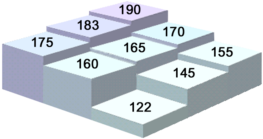
The tool estimates the surface area of each cell from that cell plus its eight neighbors, using a moving 3 × 3 window. Picture the nine cells as columns rising to their elevations, with a point at the center of the top of each column. We connect the central point to each of the eight surrounding points with straight three-dimensional lines, and connect each surrounding point to the ones on either side of it, which gives eight triangles that meet at the center of the central cell and together form a continuous surface draped over the nine cells. The length of each of those lines comes from the Pythagorean theorem: the horizontal distance between the two points (the cell size for the four orthogonal neighbors, the cell size times the square root of two for the four diagonal ones), combined with the difference in elevation.
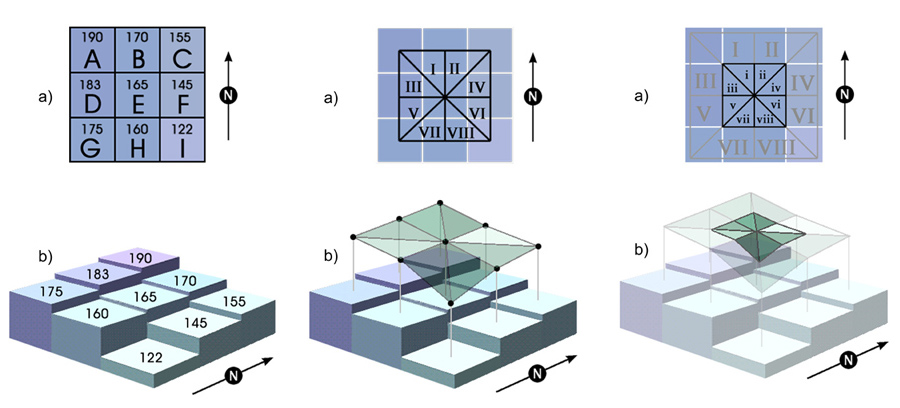
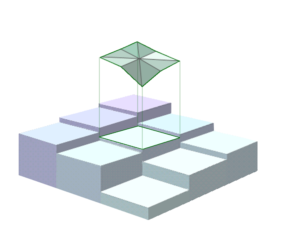
Those eight triangles cover more ground than the central cell, because each one reaches out to the centers of the neighboring cells. So the tool trims them to the cell boundary. Geometrically this is simple: the boundary of the central cell passes exactly halfway along every line that leaves its center, so the trimmed triangle is similar to the full one with every side half as long, and its area is exactly one quarter of the full triangle's area. In practice the tool works directly with the eight trimmed triangles, whose outer corners are eight points interpolated on the cell boundary: the midpoints of the four edges and the four corners of the cell. The area of each trimmed triangle comes from Heron's formula, which needs only its three side lengths:
and the cell's surface area is the sum of the eight. For the example above, with 100 m cells, the eight trimmed triangles come to 1,276.3, 1,265.5, 1,273.1, 1,280.9, 1,274.0, 1,306.8, 1,265.5 and 1,338.7 square meters, for a total of 10,280.8 m². The flat area of the cell is 100 m × 100 m = 10,000 m², so the surface ratio is 1.028: this cell holds about 2.8% more ground than its footprint. (The paper reports 10,280.48 m²; the small difference is rounding in the paper's printed tables.)
Two ways to interpolate the corners
The four edge midpoints are easy: the elevation halfway between two cell centers is the mean of the two, and that is what both corner methods use. The four corners of the cell are a genuine choice, because each corner is shared by four cells. The Diagonal midpoint (2 cells, original method) option sets the corner elevation to the mean of the focal cell and its diagonal neighbor, which is exactly what the halved-triangle construction in the 2004 paper does and exactly what the legacy DEM Surface Tools computed. The Corner average (4 cells) option instead averages all four cells that share the corner, which is the true bilinear estimate of the elevation at that point and therefore the more accurate interpolation. On a perfectly planar slope the two give identical results; they differ only where the surface curves. In the example above, the corner average gives 10,225.8 m² and a ratio of 1.023 instead of 1.028, a little lower because averaging four cells smooths the corners slightly. Use the original method if you need to reproduce results from the older tools exactly, and the corner average otherwise.
Why not compute surface area from slope?
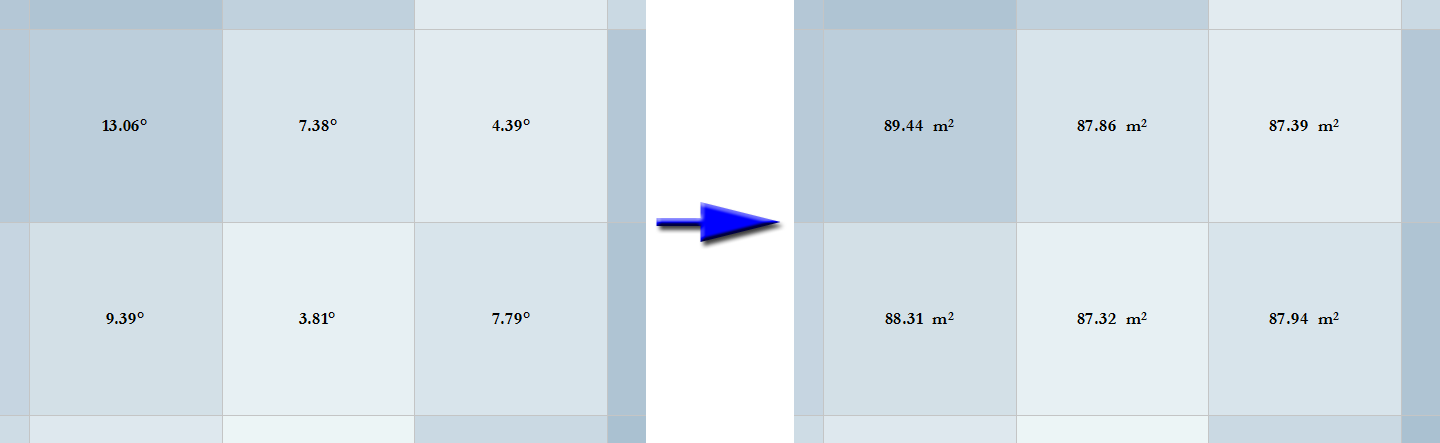
Joe Berry described a simpler route in his Beyond Mapping column (Berry 2002): a tilted cell's area is its flat area divided by the cosine of its slope angle, so a surface area raster is one map-algebra expression away from a slope raster. I have always liked Joe Berry; his columns were some of the things that inspired me to get into GIS. But this cosine method has a problem that the About page describes in detail: nearly every slope algorithm, including the one in the ArcGIS Slope tool, ignores the elevation of the central cell. Wherever the central cell sits above or below the plane of its neighbors, the true surface area is larger than the cosine estimate, and the cosine method is only exactly right in the rare case where every cell lies precisely on the gradient of its neighbors. It therefore tends to underestimate surface area, and it produces a raster perfectly correlated with slope, so you would not want both in one model. For the example cell above, Horn's (1981) slope is 12.5° and the cosine method gives 10,243 m² against the eight-triangle 10,281 m²; the gap is small on a fairly smooth cell like this one and grows with the roughness the method cannot see.
The surface-fitting algorithms of the newer Surface Parameters tool do not help here either: a surface fitted to a symmetric window is just as blind to the central cell as Horn's method when it comes to slope (the About page explains why), and the parallel-ridge and checkerboard surfaces shown there come out perfectly flat under it too.
Geographic DEMs
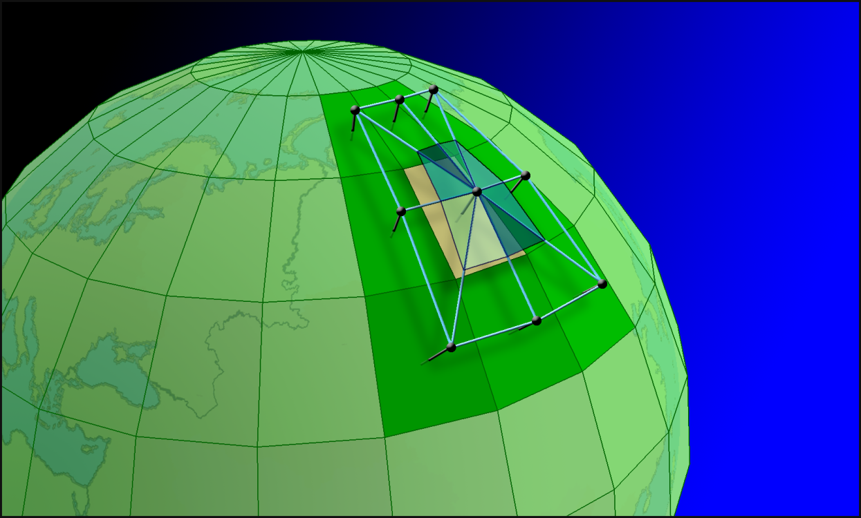
Most tools that work with elevation quietly assume the DEM is projected, with square cells of a known size in meters or feet. This tool does not require that. On a geographic DEM the sixteen distances that define the eight triangles are recomputed for every row of the raster as chord lengths on the spheroid, and the flat area of each cell is its true area on the spheroid at that row's latitude, which shrinks toward the poles. Surface areas, ratios and flat areas are therefore correct at any latitude without projecting the DEM first, and you avoid the resampling that projection imposes on a raster (see Projecting Rasters). Projected DEMs use their constant planar cell dimensions. The trapezoidal cells are also a reason to be cautious about the cosine method on geographic data: I am not sure it is appropriate for trapezoidal cells, whereas the triangles are unambiguous.
Local detrending: a third-generation surface ratio
The surface ratio is a first-generation ruggedness index in the terms of Dilts et al. (2023): it is correlated with slope, so a smooth but steep hillside scores as rough. That is exactly right if steepness is part of what you mean by roughness, and exactly wrong if you want to know how bumpy the surface is regardless of its tilt. For the second case, turn on Remove smooth topography first. The tool then smooths the DEM with a circular neighborhood mean of the radius you set (the default of 1.5 cells is exactly a 3 × 3 mean, the smoothing Dilts et al. used), subtracts that smoothed surface from the original, and runs the eight-triangle computation on the residual. What is left in the residual is only the fine-scale variation: a smooth slope becomes flat, a smooth ridgeline becomes flat, and only bumps smaller than the smoothing radius survive. The surface ratio of that residual is what Dilts et al. call SAPR-L, the local variant, and it passes all three of their tests for an ideal ruggedness index: independent of slope, unaffected by smooth folding, and rising only with true surface roughness.
In this mode the surface ratio is the output you want. The surface area and flat area rasters describe the detrended residual surface rather than the real terrain and are rarely of interest, and since detrending changes only elevations it has no effect at all on the flat area, so the option is available only when you have asked for a surface area or surface ratio output. The smoothing radius is the scale control: a larger radius removes broader topography before the roughness is measured, so hills a few cells across count as roughness at a 10-cell radius and vanish at a 1.5-cell radius.
A tour of the dialog
The example runs the tool on a 30 m DEM of a stretch of the Grand Canyon, from the South Rim across the inner gorge to the North Rim: about 2,000 m of relief, with the Colorado River at the bottom and stacked cliff bands on both walls. I chose it because it is about as rugged as terrain gets, which makes the outputs easy to read, and, as you will see, it also produces some numbers well outside the ranges I quoted above. Plus, I just like the Grand Canyon and enjoy opportunities to show images of it.
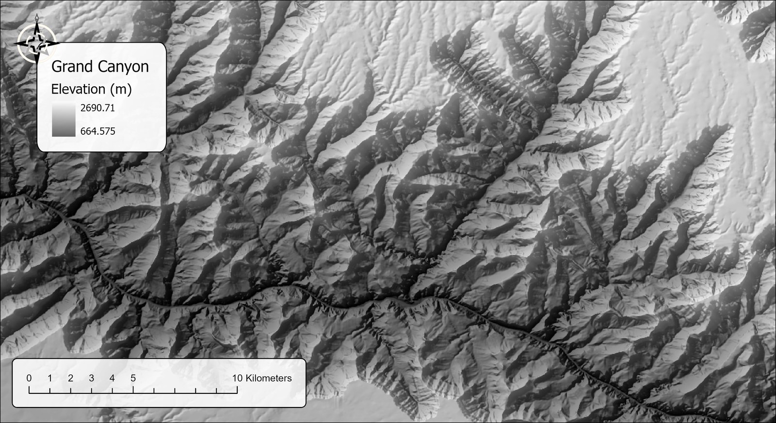
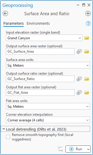
The dialog asks for the DEM and then for any combination of the three outputs. Each area output has its own units (square meters, square feet, hectares, acres, square kilometers or square miles), so you can have surface area in acres and flat area in hectares if that suits your report; the ratio is unitless. The Elevation units setting matters more than it looks: the triangles combine horizontal distances with elevation differences, so the two must be in the same unit, and with a DEM in feet treated as meters every elevation difference would be 3.28 times too large, badly inflating the areas. The tool reads the units from the DEM's vertical coordinate system when it has one and locks the setting; it assumes meters for geographic DEMs; and it asks you only when the DEM does not say. Then come the corner method and the detrending options described above.
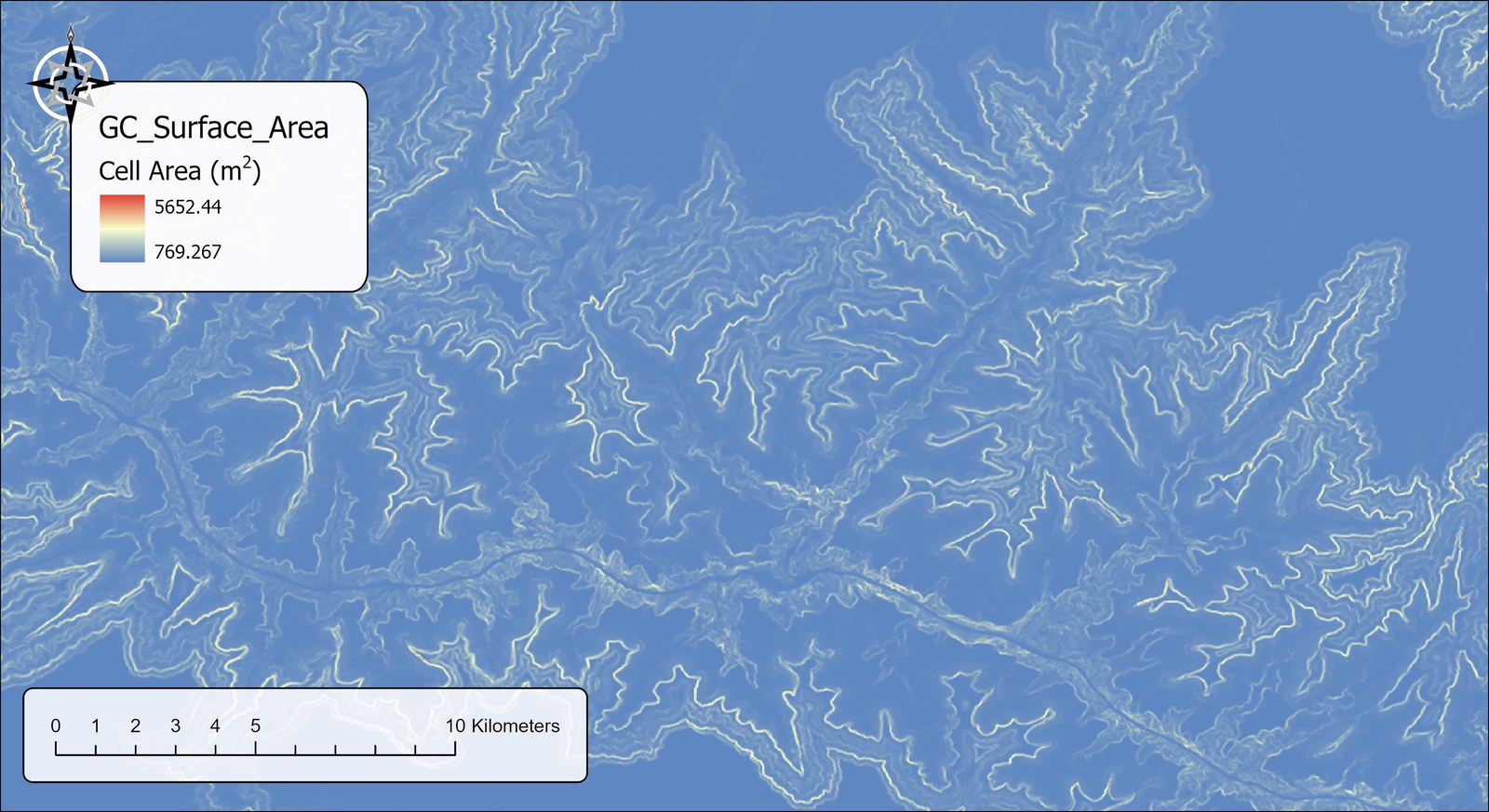
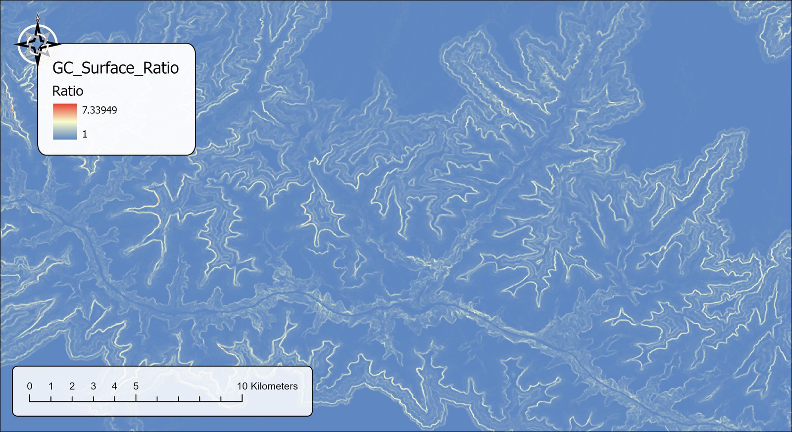
I said above that surface ratios rarely climb past 2 or 3, and here the legend tops out at 7.34, so a word about that. The Grand Canyon is an extreme example, chosen for that reason. Its walls are built of near-vertical cliff bands: the largest difference between two adjacent cells of this DEM is 275 m, and more than 16,000 adjacent pairs differ by 100 m or more. A cell whose eight triangles lean across a drop like that genuinely does hold seven times its footprint in surface. Those cells are the thin red lines along the cliffs; look at how much of the map is blue. Across most of this map the ratio stays under 1.5 (86% of cells), and values above 3 make up only 1.3% of cells. If your legend tops out at 7 on a landscape that is not the Grand Canyon, suspect the elevation units before you suspect the terrain.
The outputs are floating-point rasters. Surface area and surface ratio are NoData wherever any of the nine cells in the window is NoData, and along the outer edge of the raster, where the window is incomplete; the flat area raster is written for every cell, since it does not depend on elevations at all. Each output carries statistics, a histogram and bilinear pyramids, so it draws correctly the moment it reaches the map. A blue-yellow-red stretch is applied by default to the surface area and surface ratio outputs; the flat area raster is left with Pro's default symbology. Outputs may go into a geodatabase or a folder; in a folder, a name without an extension becomes a GeoTIFF, and you may type .tif or .img explicitly. Formats that cannot hold 32-bit floating-point values are rejected with a clear message.
The detrended surface ratio on the same canyon
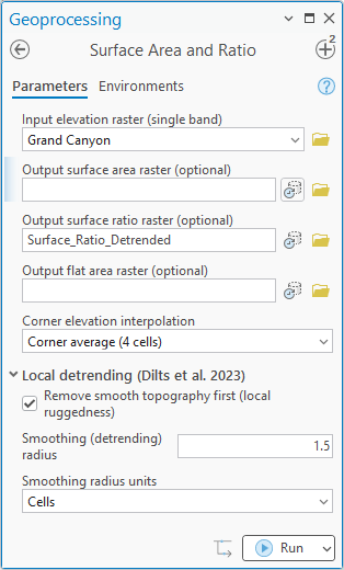
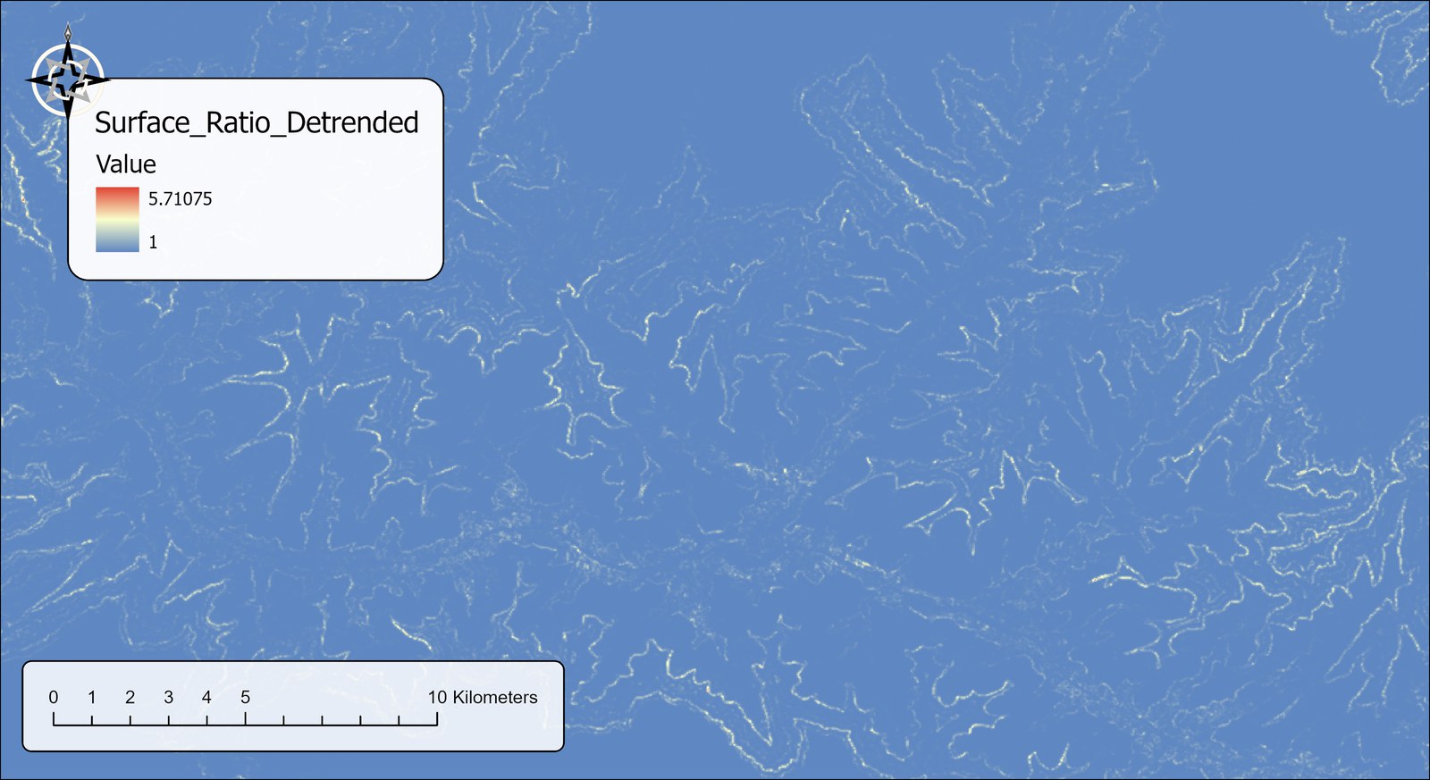
Notice that only the surface ratio was requested this time, and that is deliberate. Detrending subtracts the smoothed terrain from the DEM before the triangles are built, so the surface the tool measures is no longer the canyon but a residual: a thin sheet of bumps and dips around zero. The surface area of that sheet is a real number, but it is the area of the residual, not of the land, and nobody wants it in acres. The flat area is not affected by detrending at all, since it depends on cell geometry and not on elevation. The ratio, on the other hand, is the quantity Dilts et al. (2023) call SAPR-L: how much extra surface the bumps add to a locally flattened landscape. So when detrending is on, ask for the ratio and leave the two area outputs blank.
The extremes come down after detrending, and it is worth thinking about why. The most likely reason is that a cliff cell scored 7 in the first run mostly because of its tilt: its eight triangles reach from the top of the cliff to the bottom, and nearly all of that area is the smooth face itself. A 3 × 3 mean removes most of that tilt, and a smooth steep face, once flattened, is nearly a plane with a ratio near 1. What survives is the roughness that a 3 × 3 mean cannot smooth away, and the sharp brink of a cliff is the best example: the mean straddles the edge, so the residual there is still a step, only a smaller one. That would explain why the cliff lines are still visible, thinner and fainter, and why the maximum drops rather than vanishing. The broad, bright bands on the smooth cliff faces are gone because they were steepness, and steepness is precisely what the third-generation index is designed to ignore.
The tool normally works through the DEM in strips, so the size of the DEM is not a concern. With the detrending option on, though, it holds the whole DEM in memory at once, and the memory it needs grows with the number of cells. On a very large one the tool may need more memory than your computer has free, and then one of two things happens: Windows starts using the disk as overflow memory and the tool slows to a crawl, or the tool stops with an out-of-memory error. There is no fixed limit; it depends on how much memory your computer has free. If a DEM is too large to detrend, clip it to the area you need first.
Environment settings
Each output matches the input DEM exactly: same extent, cell size and coordinate system. The Processing Extent, Snap Raster, Cell Size, Output Coordinate System and Mask environments are deliberately not applied, so that the delivered raster is the grid the surface areas were computed on; project, clip or resample the finished raster yourself if you need to. Pyramids are always built with bilinear resampling regardless of the Pyramid environment. The triangles are only as good as the elevations they connect, which is the reason to compute at the DEM's own resolution and coordinate system.
ModelBuilder
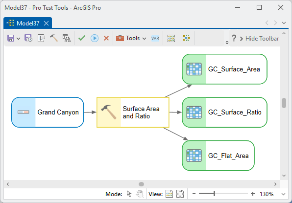
Parameters
| Label | Explanation | Data type |
|---|---|---|
| Input elevation raster (single band)Required · in_raster | The DEM. Must be single band; projected or geographic. Choose a layer from the map or browse to a dataset. | Raster Layer |
| Output surface area raster (optional)Optional · out_area | The three-dimensional surface area within each cell, in the surface area units. At least one of the three outputs is required. | Raster Dataset |
| Surface area unitsOptional · area_units | Sq. Meters, Sq. Feet, Hectares, Acres, Sq. Kilometers or Sq. Miles. Default Sq. Meters; enabled only when the matching output is named. | String |
| Output surface ratio raster (optional)Optional · out_ratio | Surface area divided by flat area: unitless, 1 on level ground, larger with slope and convolution (or, with detrending on, with fine-scale roughness alone). | Raster Dataset |
| Output flat area raster (optional)Optional · out_flat | The planimetric area of each cell in the flat area units. Constant on projected rasters; varies by row on geographic rasters. Valid for every cell, even NoData areas of the DEM. | Raster Dataset |
| Flat area unitsOptional · flat_units | Sq. Meters, Sq. Feet, Hectares, Acres, Sq. Kilometers or Sq. Miles. Default Sq. Meters; enabled only when the matching output is named. | String |
| Elevation unitsOptional · elev_units | Meters or Feet. Filled in and locked from the DEM's vertical coordinate system when it has one; geographic DEMs are assumed to be in meters; you are asked only when the DEM does not say. | String |
| Corner elevation interpolationRequired · corner_method | Diagonal midpoint (2 cells, original method) reproduces the 2004 paper and the legacy DEM Surface Tools; Corner average (4 cells) is the true bilinear estimate and the more accurate choice. Identical on planar slopes. Diagonal midpoint is the default; the dialog remembers the last choice made, as it does for the other options. | String |
| Remove smooth topography first (local ruggedness)Optional · detrend | Subtract a circular neighborhood mean of the DEM before computing, so the surface ratio becomes the local variant SAPR-L of Dilts et al. (2023). Available only when a surface area or surface ratio output is requested. Off by default. | Boolean |
| Smoothing (detrending) radiusOptional · detrend_radius | Radius of the smoothing mean. The default 1.5 cells is exactly a 3 × 3 mean; larger radii remove broader topography. Used only when detrending is on. | Double |
| Smoothing radius unitsOptional · detrend_units | Cells, Meters, Kilometers, Feet or Miles; ground units are converted to cells from the cell size, per row on the spheroid for geographic DEMs, where the east–west radius is rounded to whole cells row by row. | String |
Python
import arcpy
arcpy.ImportToolbox(r"C:\path\to\JennessEnterprisesTools.pyt")  # your install path
# Surface area in acres plus the roughness ratio, with the improved corners.
arcpy.jenness.SurfaceAreaRatio(
    in_raster=r"C:\Project\Elev.gdb\DEM",
    out_area=r"C:\Project\Elev.gdb\DEM_SurfArea",
    out_ratio=r"C:\Project\Elev.gdb\DEM_SurfRatio",
    area_units="Acres", elev_units="Meters",
    corner_method="Corner average (4 cells)")
# The local (detrended) surface ratio, SAPR-L, with a 3 x 3 smoothing mean.
arcpy.jenness.SurfaceAreaRatio(
    in_raster=r"C:\Project\Elev.gdb\DEM",
    out_ratio=r"C:\Project\Elev.gdb\DEM_SAPRL",
    elev_units="Meters",
    corner_method="Corner average (4 cells)",
    detrend=True, detrend_radius=1.5, detrend_units="Cells")
Recommended citation
Credits and references
By Jeff Jenness, Jenness Enterprises (www.jennessent.com), modernizing the surface area functions of his DEM Surface Tools for ArcGIS extension and his Surface Areas and Ratios from Elevation Grid extension for ArcView 3.x. The local-detrending option follows Dilts et al. (2023).
- Berry, J. K. 2002. Use surface area for realistic calculations. Geoworld 15(9):20–21. innovativegis.com/basis/MapAnalysis/Topic11
- Bowden, D. C., G. C. White, A. B. Franklin, and J. L. Ganey. 2003. Estimating population size with correlated sampling unit estimates. Journal of Wildlife Management 67:1–10. doi.org/10.2307/3803055
- Dilts, T. E., M. E. Blum, K. T. Shoemaker, P. J. Weisberg, and K. M. Stewart. 2023. Improved topographic ruggedness indices more accurately model fine-scale ecological patterns. Landscape Ecology 38:1395–1410. doi.org/10.1007/s10980-023-01646-6
- Horn, B. K. P. 1981. Hill shading and the reflectance map. Proceedings of the IEEE 69:14–47. doi.org/10.1109/PROC.1981.11918
- Jenness, J. 2002. Surface Areas and Ratios from Elevation Grid (surfgrids.avx) extension for ArcView 3.x, v. 1.2. Jenness Enterprises. jennessent.com/arcview/surface_areas.htm
- Jenness, J. S. 2004. Calculating landscape surface area from digital elevation models. Wildlife Society Bulletin 32:829–839. jennessent.com/downloads/WSB_32_3_Jenness.pdf; doi.org/10.2193/0091-7648(2004)032[0829:CLSAFD]2.0.CO;2
- Jenness, J. 2013. DEM Surface Tools for ArcGIS (surface_area.exe), build 2.1.375. Jenness Enterprises. jennessent.com/arcgis/surface_area.htm
Licensing information
Works at every ArcGIS Pro license level (Basic, Standard, Advanced). No extension licenses are required; the surface areas are computed internally, without Spatial Analyst or 3D Analyst.
Related tools and pages
- About Topographic Roughness — choosing among the nine roughness measures.
- Arc-Chord Ratio (ACR) — the same surface area divided by a tilted reference plane, so slope drops out.
- Vector Ruggedness Measure (VRM) — roughness as variation in the direction cells face.
- Terrain Ruggedness Index (TRI) — roughness as elevation differences between neighbors.
- Topography along Lines — surface length and surface ratio of a polyline rather than a cell.
- Projecting Rasters — why this tool works on geographic DEMs directly, and how to project a DEM properly when you must.