

Slope Position Classification
Summary
Classifies a DEM into slope-position classes — valley bottom, lower, middle and upper slope, flat, and ridge — from a Topographic Position Index (TPI; Weiss 2001, after Guisan et al. 1999) plus slope, using a saved classification system. TPI is simply the difference between a cell's elevation and the mean elevation of a neighborhood around it: positive on hills and ridges, negative in valleys and channels, near zero on flats and mid-slopes, with slope telling the last two apart. The TPI and slope are computed internally from the DEM, with no Spatial Analyst extension, or you may supply pre-computed rasters. The neighborhood radius is often one of the most difficult parameters to estimate because we rarely have good data to guide us. The same point can be a valley bottom at one scale and a hilltop at another, and both are valid for different species or different questions.
Scale, units and classification systems
Neighborhood size is the scale of the analysis. A small neighborhood picks out local hills and hollows; a large one picks out broad ridges and valleys, and a point that is a valley bottom at one scale can be a hilltop at another. Choose the scale that matters for your question: a wide-ranging animal responds to major ridgelines hundreds of feet high, not to minor bumps underfoot, so a larger neighborhood suits it. The radius may be given in cells or in ground units, as a full circle or as an annulus that considers only a band of distances. On a geographic (latitude/longitude) DEM a ground radius is worked out per row on the spheroid, rounded east-west to a whole number of cells for each band of rows, so the neighborhood stays a circle on the ground to within about half a cell at any latitude.
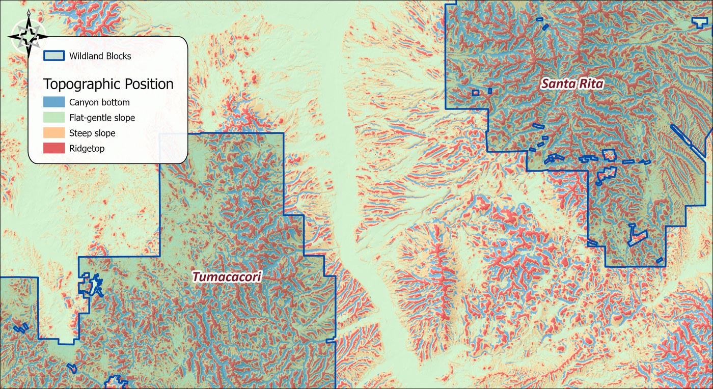
Classification systems are reusable, named rule sets: the class thresholds, names and colors, saved as JSON in a per-user location that survives add-in reinstalls. The bundled defaults are a 6-class slope-position system adapted from Weiss (2001), Dickson and Beier's 4-class system, the Corridor Designer 4-Class Topographic Position system from the CorridorDesigner toolbox tutorial (Majka et al. 2007) (raw TPI, cells at least 12 m below their neighborhood mean are canyon bottom, at least 12 m above it are ridgetop, and everything between splits at a 6° slope into flat-gentle and steep slope), and the Land Facet Corridor Designer 3-Class Topographic Position system, the canyons, slopes and ridges that land facets are built within (raw TPI at −6 and +6 m, no slope criterion). New systems, including per-class colors that symbolize the output when it reaches the map, are authored in the Classification System Builder. Classification is applied cell by cell in one pass; a class is the AND of its criteria, and where classes overlap the lowest class value wins.
Raw versus standardized TPI. Raw TPI is in the DEM's elevation units, so a threshold is absolute: a 100 m hill is read the same way everywhere. That is usually the right choice for ecological questions, where absolute relief is what an animal experiences. Standardized TPI expresses the value relative to the variability of the terrain (Weiss's own default), so a 1 m bump on a plain and a 100 m hill in the mountains can fall in the same class; useful when a classification must adapt to each landscape, but ecologically misleading if you are expecting a 100 m hill to be treated the same everywhere. Each classification system records which form its thresholds assume, the dialog defaults to that form when you pick a system, and the tool warns, but still runs, if you override it.
Both choices, the neighborhood and the thresholds of the system, can be tried before a full run with the TPI Neighborhood Sampler: a snapshot of the DEM in the map view, a slider for the radius, a slider for a threshold in raw or neighborhood standard deviation units, and a pin that shows at which radii a chosen hill or valley falls into the class. What it finds goes into the on-the-fly neighborhood here and into the system's criteria in the Classification System Builder.
How the classes are defined
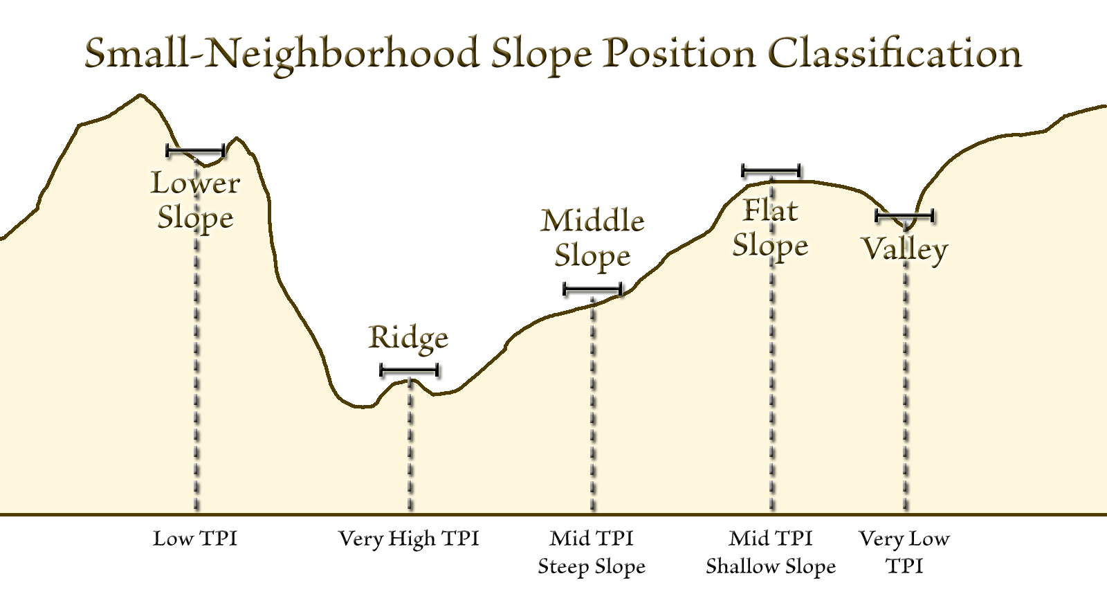
A slope-position class is a range of TPI, with slope added only where TPI alone cannot decide. A cell well above its neighborhood mean is a ridge; a cell well below it is a valley; and a cell near the mean is either flat ground or an even mid-slope, which slope tells apart. The profile below, from the manual of the ArcView 3.x TPI extension (Jenness 2006), shows how five of the classes of Weiss (2001) fall on a cross-section; the maps after it show all six.
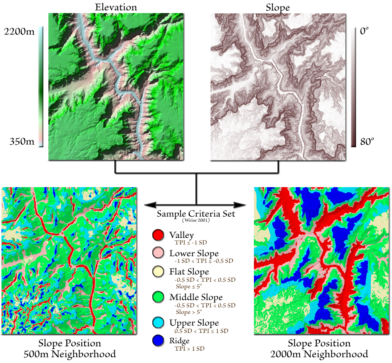
Six slope-position systems ship with the add-in. Three are adapted from the Weiss six-class scheme, one in each of the three TPI forms, two are four-class schemes from cougar and corridor work, and one is the three-class scheme of the land facet method (and remember that you can easily make your own system with the Classification System Builder). The table gives each system exactly as its file defines it. Where a cell satisfies more than one class, the lowest class value wins; none of the bundled systems has overlapping classes, so what happens to a cell exactly at a break is decided by the ≤, < and ≥ signs in the rules. In the Weiss systems a cell exactly at −1 is a Valley, at −0.5 a Lower Slope, at 0.5 or 1 an Upper Slope (the Flat and Middle Slope ranges are open at both ends), and above 1 a Ridge, with the same pattern at the raw and percentile breaks.
| System | Value | Class | Rule |
|---|---|---|---|
| Weiss 6-Class Slope Position TPI in neighborhood standard deviations; slope in degrees |
1 | Valley | TPI ≤ −1 |
| 2 | Lower Slope | −1 < TPI ≤ −0.5 | |
| 3 | Flat Slope | −0.5 < TPI < 0.5 and slope ≤ 5° | |
| 4 | Middle Slope | −0.5 < TPI < 0.5 and slope > 5° | |
| 5 | Upper Slope | 0.5 ≤ TPI ≤ 1 | |
| 6 | Ridge | TPI > 1 | |
| Weiss 6-Class Slope Position, using Raw TPI values TPI in elevation units; slope in degrees |
1 | Valley | TPI ≤ −20 |
| 2 | Lower Slope | −20 < TPI ≤ −5 | |
| 3 | Flat Slope | −5 < TPI < 5 and slope ≤ 5° | |
| 4 | Middle Slope | −5 < TPI < 5 and slope > 5° | |
| 5 | Upper Slope | 5 ≤ TPI ≤ 20 | |
| 6 | Ridge | TPI > 20 | |
| Weiss 6-Class Slope Position, using Percentile TPI values TPI in percentile units (0–100); slope in degrees |
1 | Valley | TPI ≤ 10 |
| 2 | Lower Slope | 10 < TPI ≤ 45 | |
| 3 | Flat Slope | 45 < TPI < 55 and slope ≤ 5° | |
| 4 | Middle Slope | 45 < TPI < 55 and slope > 5° | |
| 5 | Upper Slope | 55 ≤ TPI ≤ 90 | |
| 6 | Ridge | TPI > 90 | |
| Dickson & Beier 4-Class Slope Position TPI in elevation units; slope in degrees |
1 | Ridgeline | TPI ≥ 8 |
| 2 | Steep Slope | −8 < TPI < 8 and slope ≥ 6° | |
| 3 | Gentle Slope | −8 < TPI < 8 and slope < 6° | |
| 4 | Canyon Bottom | TPI ≤ −8 | |
| Corridor Designer 4-Class Topographic Position TPI in elevation units; slope in degrees |
1 | Canyon bottom | TPI ≤ −12 |
| 2 | Flat-gentle slope | −12 < TPI < 12 and slope ≤ 6° | |
| 3 | Steep slope | −12 < TPI < 12 and slope > 6° | |
| 4 | Ridgetop | TPI ≥ 12 | |
| Land Facet Corridor Designer 3-Class Topographic Position TPI in elevation units; no slope |
1 | Canyons | TPI ≤ −6 |
| 2 | Slopes | −6 < TPI ≤ 6 | |
| 3 | Ridges | TPI > 6 |
The Weiss system is adapted from the six-class scheme of his 2001 poster. As bundled here its thresholds are applied to TPI in standard deviations of the elevations within each cell's own neighborhood; the poster itself standardized each whole TPI raster to z-scores, a form the tools do not compute (see About TPI). The raw variant keeps the same shape with thresholds of ±5 and ±20 elevation units, and the percentile variant places its breaks at the 10th, 45th, 55th and 90th percentiles of the neighborhood, the percentile form of TPI described by Wilson and Gallant (2000). Because a cell is counted in its own circular neighborhood, its percentile can reach at most 100(n − 1)/n for n cells, 88.9 in the 9 cells of a 1.5-cell radius, so the Ridge class (above 90) needs a radius of at least 2 cells; the tool warns whenever a percentile class threshold cannot be reached with the neighborhood used. Both variants are meant as starting points: raw thresholds are absolute relief and should be adjusted to the DEM and the question. The Dickson and Beier system follows their study of topographic position and cougar movement in southern California (Dickson and Beier 2007), with raw thresholds of ±8 and a 6° slope split; its codes run from ridgeline (1) to canyon bottom (4). The Corridor Designer system reproduces the topographic position raster of the CorridorDesigner tutorial, with ±12 thresholds and the same 6° split, and its codes run the other way, from canyon bottom (1) to ridgetop (4); the two are not interchangeable in a model that keys on the codes.
Two ways to supply the TPI and slope. The TPI and slope source setting at the top of the dialog chooses between calculating both from a DEM, with the neighborhood, TPI type, slope method and slope units set in the dialog, and classifying TPI and slope rasters that already exist, for example outputs of the Topographic Position Index tool or rasters saved by an earlier run of this one. In either case the tool classifies the values it is given as they are; it never converts a raw TPI to standardized units or back. What it does check is whether the values match what the system expects. Rasters written by these tools carry their TPI type, their neighborhood radius and their slope units in their metadata, and the tool reads those stamps; for a raster made elsewhere, the two Declare dropdowns let you state its type and units. If the type or the units do not match the system's thresholds, the tool warns, writes the warning into the output's metadata as well, and still runs. The warning compares kinds only, raw, standard-deviation or percentile: the DEM-scale and experimental outputs of the Topographic Position Index tool both count as standard-deviation kinds and pass a system written for the neighborhood-standardized TPI without a warning.
A tour of the dialog
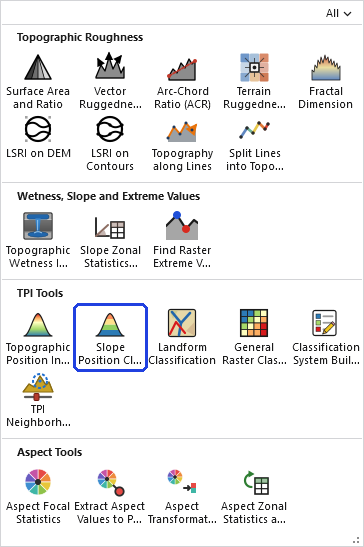
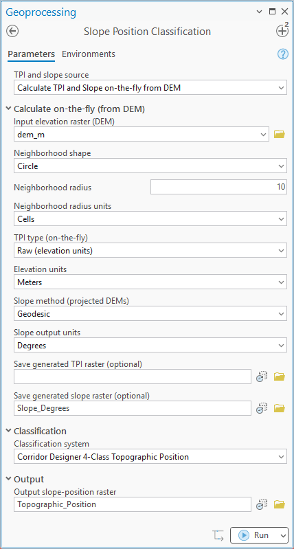
The example is the first step of the Land Facet Tutorial, where topographic position is the first-pass classification that the land facets are then built within. The Corridor Design Tutorial runs the same tool with a 200 m radius to make the topographic position factor of a habitat suitability model.
Classifying existing rasters: a Grand Canyon example
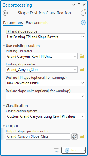
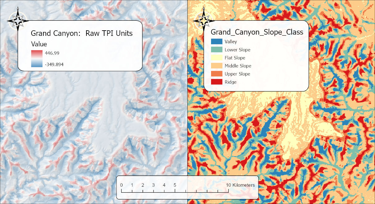
The second example classifies rasters that already exist: the raw TPI of the Walhalla Plateau in the Grand Canyon, computed with a 500 m circular neighborhood on the Topographic Position Index page, and a slope raster of the same area. With Use Existing TPI and Slope Rasters chosen, the DEM and neighborhood settings drop out of the dialog, and only the two rasters, their optional Declare dropdowns, the classification system and the output remain.
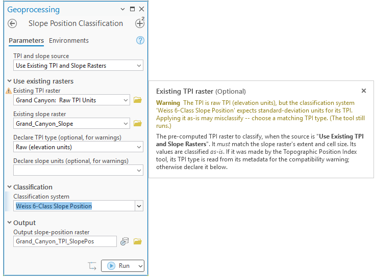
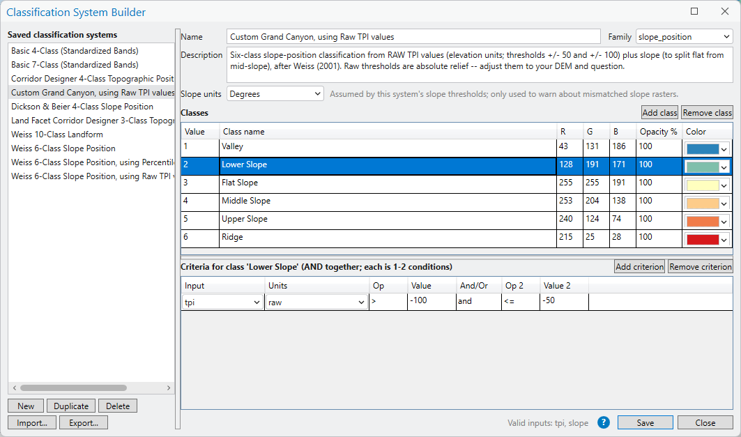
The bundled raw-TPI version of the Weiss scheme would match the units, but its thresholds of 5 and 20 m are far too small for a canyon where the TPI runs from −350 to +447 m, where even modest side canyons and spurs would clear them. This is exactly the case the Classification System Builder is for. Starting from the raw-TPI Weiss system and widening its thresholds to ±50 and ±100 m gives a system suited to Grand Canyon relief, saved under its own name so the bundled one stays as it was.
The tool holds the whole raster in memory at once, so the memory it needs grows with the number of cells. On most rasters that is no concern. On a very large one the tool may need more memory than your computer has free, and then one of two things happens: Windows starts using the disk as overflow memory and the tool slows to a crawl, or the tool stops with an out-of-memory error. There is no fixed limit; it depends on how much memory your computer has free. If a raster is too large, clip it to the area you need first.
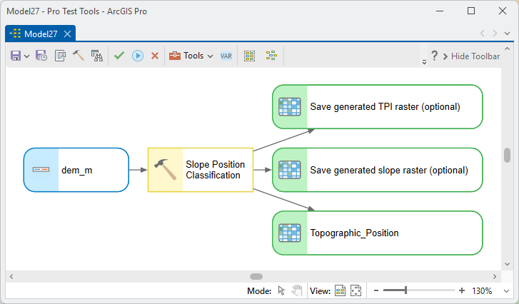
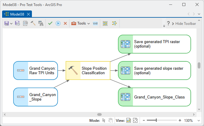
ModelBuilder
Parameters
| Label | Explanation | Data type |
|---|---|---|
| TPI and slope sourceRequired · tpi_source | Calculate TPI and Slope on-the-fly from DEM (default) computes both from the DEM with the settings below; Use Existing TPI and Slope Rasters classifies rasters you already have, as they are. | String |
| Input elevation raster (DEM)Optional · in_raster | Single-band DEM, projected or geographic; required when calculating on the fly. | Raster Layer or Dataset |
| Neighborhood shapeRequired · nb_shape | Circle (all cells within the radius) or Annulus (a ring between an inner and outer radius). Default Circle. | String |
| Neighborhood radiusRequired · nb_outer | The (outer) radius: the scale of the analysis. Default 10. | Double |
| Neighborhood inner radius (annulus only)Optional · nb_inner | For an annulus, cells nearer than this are excluded. | Double |
| Neighborhood radius unitsRequired · nb_units | Cells, or a ground unit (meters, kilometers, feet, miles) converted from the cell size; per row on the spheroid for geographic DEMs. Default Cells. | String |
| TPI type (on-the-fly)Required · tpi_type | Raw (elevation units), Neighborhood standard deviation or Percentile. Defaults to what the chosen system expects (Neighborhood standard deviation for the Weiss 6-class); a mismatch warns and still runs. | String |
| Elevation unitsOptional · elev_units | Meters or feet, for the slope calculation; detected and locked when the DEM has a vertical coordinate system. | String |
| Slope method (projected DEMs)Optional · slope_method | Planar (matches Esri's Slope tool) or Geodesic; geographic DEMs are always geodesic. Default Planar. | String |
| Slope output unitsRequired · slope_units | Degrees or percent rise; defaults to the system's assumption (Degrees for the bundled systems) and warns on a mismatch. | String |
| Save generated TPI raster (optional)Optional · save_tpi | Keep the intermediate TPI raster, stamped with its TPI type. Blank keeps it in memory only. | Raster Dataset |
| Save generated slope raster (optional)Optional · save_slope | Keep the intermediate slope raster, stamped with its units. | Raster Dataset |
| Existing TPI rasterOptional · in_tpi | When using existing rasters: the TPI to classify, as is. Must have the same number of rows and columns as the slope raster; the tool checks the dimensions, not the extent. | Raster Layer or Dataset |
| Existing slope rasterOptional · in_slope | When using existing rasters: the slope raster; required when the system uses slope. | Raster Layer or Dataset |
| Declare TPI type (optional, for warnings)Optional · declare_tpi_type | What kind of TPI an existing raster holds, when its metadata does not say; used only for the compatibility warning. | String |
| Declare slope units (optional, for warnings)Optional · declare_slope_units | Degrees or percent for an existing slope raster, when its metadata does not say; warnings only. | String |
| Classification systemRequired · system | The saved system to apply: thresholds, names and colors. Picking one sets the TPI-type and slope-unit defaults. Default Weiss 6-Class Slope Position. | String |
| Output slope-position rasterRequired · out_raster | Integer class raster with a Value / Class_Name table and the system's color map. Cells matching no class are unclassified. Any unit warnings are written into its metadata. | Raster Dataset |
Python
import arcpy
arcpy.ImportToolbox(r"C:\path\to\JennessEnterprisesTools.pyt")  # your install path
arcpy.jenness.SlopePositionClassification(
    tpi_source="Calculate TPI and Slope on-the-fly from DEM",
    in_raster=r"D:\tutorial.gdb\dem_m",
    nb_shape="Circle", nb_outer=10, nb_units="Cells",
    tpi_type="Raw (elevation units)", elev_units="Meters",
    slope_method="Geodesic", slope_units="Degrees",
    save_slope=r"D:\tutorial.gdb\Slope_Degrees",
    system="Corridor Designer 4-Class Topographic Position",
    out_raster=r"D:\tutorial.gdb\Topographic_Position")

# Classify TPI and slope rasters that already exist, as they are.
# The declare_* arguments are optional; rasters made by these tools
# carry their type and units in their metadata.
arcpy.jenness.SlopePositionClassification(
    tpi_source="Use Existing TPI and Slope Rasters",
    in_tpi=r"D:\tutorial.gdb\dem_TPI", in_slope=r"D:\tutorial.gdb\Slope_Degrees",
    declare_tpi_type="Neighborhood standard deviation",
    declare_slope_units="Degrees",
    system="Weiss 6-Class Slope Position",
    out_raster=r"D:\tutorial.gdb\Slope_Position_Weiss")
The list-driven parameters take these strings exactly:
tpi_source is "Calculate TPI and Slope on-the-fly from
DEM" or "Use Existing TPI and Slope Rasters";
nb_shape is "Circle" or "Annulus";
nb_units is "Cells", "Meters",
"Kilometers", "Feet" or
"Miles"; tpi_type is "Raw (elevation
units)", "Neighborhood standard deviation" or
"Percentile"; elev_units is
"Meters" or "Feet"; slope_method
is "Planar" or "Geodesic";
slope_units and declare_slope_units are
"Degrees" or "Percent";
declare_tpi_type adds "DEM-scale standard
deviation" to the three TPI types; and system is the
name of any slope-position system in the store, bundled or your
own. The names of the
systems on your computer are listed in the
Classification System
Builder; they are also the "name" entries of the
JSON files in
%LOCALAPPDATA%\JennessEnterprises\WildlifeTools\classification_systems\,
but if you look them up there, take care not to change anything: an
edited file can leave a system unreadable.
Recommended citation
Credits and references
By Jeff Jenness, Jenness Enterprises (www.jennessent.com), modernizing his Topographic Position Index extension for ArcView 3.x. The Corridor Designer 4-class system reproduces the Create Topographic Position Raster tool by Dan Majka in the CorridorDesigner toolbox (Beier, Majka and Jenness 2007).
- Beier, P., D. Majka, and J. Jenness. 2007, revised 2026. Designing wildlife corridors with ArcGIS: ArcGIS Pro edition. Workshop book, revised by J. Jenness for the Corridor Designer Tools of the Wildlife and Forestry Tools add-in. Available at: CorridorDesigner_WorkshopBook_2026_ArcGISPro.pdf (5 MB)
- Dickson, B. G., and P. Beier. 2007. Quantifying the influence of topographic position on cougar (Puma concolor) movement in southern California, USA. Journal of Zoology 271:270–277. doi.org/10.1111/j.1469-7998.2006.00215.x
- Guisan, A., S. B. Weiss, and A. D. Weiss. 1999. GLM versus CCA spatial modeling of plant species distribution. Plant Ecology 143:107–122. doi.org/10.1023/A:1009841519580
- Jenness, J. 2006. Topographic Position Index (tpi_jen.avx) extension for ArcView 3.x, v. 1.3a. Jenness Enterprises. jennessent.com/arcview/tpi.htm
- Majka, D., J. Jenness, and P. Beier. 2007. CorridorDesigner: ArcGIS tools for designing and evaluating corridors. Available at: corridordesign.org (archived copy at the Internet Archive)
- Weiss, A. 2001. Topographic Position and Landforms Analysis. Poster presentation, ESRI User Conference, San Diego, CA. jennessent.com/arcview/TPI_Weiss_poster.htm
- Wilson, J. P., and J. C. Gallant. 2000. Terrain analysis: principles and applications. John Wiley and Sons, New York.
Licensing information
Works at every ArcGIS Pro license level (Basic, Standard, Advanced). No extension licenses are required; the TPI and slope are computed internally, without Spatial Analyst.
Related tools and pages
- About TPI — the Topographic Position Index, scale, and the six TPI tools.
- Topographic Position Index — the TPI rasters this tool classifies, in raw, standardized and percentile forms.
- Landform Classification — ten landform classes from TPI at two scales plus slope.
- General Raster Classification — the same classification systems applied to any single raster.
- Classification System Builder — author and edit the systems this tool applies.
- Land Facet Tutorial — topographic position as the first-pass classification for land facets.
- Corridor Design Tutorial — topographic position as a habitat factor.
- Create Habitat Suitability Model
- Projecting Rasters — project the DEM with bilinear interpolation before deriving topographic position.
- TPI Neighborhood Sampler — try neighborhood sizes and thresholds on a snapshot of the DEM, with sliders, before running the tools.