

Arc-Chord Ratio (ACR)
Summary
Computes the Arc-Chord Ratio rugosity index of Du Preez (2015): each cell's three-dimensional surface area divided by the area of its plane of best fit, rather than by its flat map footprint. The ordinary surface ratio rises with slope because a tilted plane contains more surface than the footprint beneath it; ACR measures the surface against a reference plane that tilts with the terrain, so a smooth slope of any steepness scores exactly 1 and only genuine roughness raises the value. For a raster, ACR works out to the surface ratio of Jenness (2004) multiplied by the cosine of the neighborhood's best-fit slope, which is how this tool computes it. The tool is correct on geographic (latitude/longitude) DEMs and offers the local detrending of Dilts et al. (2023) for the ACR-L variant. No Spatial Analyst license is needed.
Rugosity and the problem with the flat footprint
Rugosity is the ratio of a surface's true area to some planar reference area, and in Du Preez's (2015) words it is “widely used as a measure of landscape structural complexity”; coral-reef biologists have measured it for decades with the “chain-and-tape” method, draping a chain over the reef and comparing the chain's length with the straight-line distance it covers (Risk 1972; Luckhurst and Luckhurst 1978; McCormick 1994). Risk, who was relating fish diversity to the complexity of the reef, used a fine-link chain laid eight times across each square-meter quadrat, and found that in some places four meters of chain were needed to cover one straight meter. He stretched 1,028 m of chain over the reef that way, at five hours or more per quadrat, which may make you feel better about how long a raster tool takes. Luckhurst and Luckhurst (1978) refined the method and named the result. They laid a fine-link brass chain (each link 1.5 cm long) over the reef beneath ropes strung every 50 cm across 3 × 3 m quadrats off Curaçao and Bonaire, making it “conform as closely as possible to all contours and crevices,” and called the ratio of chain length to straight-line distance the substrate rugosity index. Their values ran from 1.10 over sandy rubble to 4.60 where the reef had about 1.5 m of vertical relief and small caves, and the number of resident fish species in a quadrat rose with it (r = 0.78 at Curaçao). They also found that the relationship depended on the size of the fish. Their chain measured what they called gross reef morphology, and they predicted that the smallest species, for which the scale of the individual coral matters more, would be poorly related to it. They were: the number of species smaller than 50 mm was only weakly related to the index (r = 0.54, not significant), while the number of species larger than 50 mm was strongly related to it (r = 0.81). In their words, “the scale of the SR index may have a strong influence on the correlations.” The same is true of every index on these pages: it describes the terrain at the scale it was measured, and an animal responds to the terrain at its own.
On a DEM the natural version is the surface ratio of the Surface Area and Ratio tool: the three-dimensional area of each cell, divided by the flat area of the cell. That ratio is 1 on level ground and rises with roughness, which is what we want. It also rises with slope, which may not be. A perfectly smooth plane tilted at 30° contains 1 / cos 30° = 1.155 times the area of the footprint beneath it; at 45° the factor is 1.414; at 60° it is 2. A smooth steep hillside therefore has a surface ratio well above 1 even though there is nothing rough about it, and slope and roughness are confounded in the one number. Dilts et al. (2023) call the surface ratio a first-generation ruggedness index for exactly this reason.
The arc and the chord
Du Preez (2015) resolves the confounding with a change of reference plane. Picture a rugged surface in cross section as an arc, and the straight line joining its two ends as the chord beneath it. The traditional surface ratio measures the arc against a horizontal line, so that a tilted arc looks longer than it should. The arc-chord ratio measures it against its own chord, the line that tilts with it. In three dimensions the chord becomes the plane of best fit through the surface, and Du Preez's index is:
where the contoured area is the true three-dimensional surface area (the arc) and the denominator is the area of that surface projected orthogonally onto its best-fit plane (the chord). A smooth tilted plane is its own plane of best fit, so its ACR is exactly 1 whatever its slope; a flat plane is also 1; and a surface with bumps on it has more contoured area than its best-fit plane and an ACR above 1. In the worked example in Du Preez's Figure 1, a tilted rugged surface has a traditional rugosity of 4.31 against its horizontal footprint but an ACR of 3.21 against its best-fit plane; the difference, a factor of 0.745, is the cosine of the 41.8° tilt of the chord, and it is the part of the traditional value that was measuring slope rather than roughness.
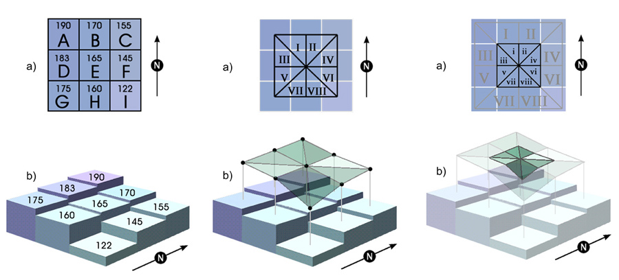
Du Preez gives the recipe for an elevation raster explicitly, and this tool follows his steps for each cell over its 3 × 3 neighborhood. The contoured area is the eight-triangle surface area of Jenness (2004): eight three-dimensional triangles connecting the cell center to eight points interpolated on the cell boundary, each measured with Heron's formula and summed. The plane of best fit is the standard 3 × 3 surface of Horn's method (Horn 1981), the same gradients that underlie the ArcGIS Slope tool, and the area of the cell projected onto that plane is the flat cell area divided by the cosine of the plane's slope. Dividing the contoured area by that tilted planar area is algebraically the same as taking the ordinary surface ratio and multiplying it by the cosine of the best-fit slope:
where is the slope of the best-fit plane. The cosine of that slope is simply the vertical component of the unit normal vector that the Vector Ruggedness Measure (Sappington et al. 2007) tool already computes for every cell, so ACR is the surface-area machinery and the VRM machinery multiplied together. Take the example cell from the Surface Area and Ratio page, the cell with elevation 165 on a 100 m DEM: its surface ratio is 1.028 and its Horn slope is 12.5°, so its ACR is 1.028 × cos 12.5° = 1.028 × 0.976 = 1.004. Almost all of that cell's extra surface came from its tilt; once the tilt is removed, the cell is very nearly a smooth plane, and ACR says so. For a smooth 30° plane the arithmetic is 1.155 × cos 30° = 1.155 × 0.866 = 1.000 exactly.
What ACR sees, and what it does not
ACR is a second-generation index in the scheme of Dilts et al. (2023), alongside VRM: it passes the tilted-plane test, since a smooth slope of any steepness scores 1, so slope and roughness can enter a model as separate variables. Like VRM it still fails the smooth-fold test. A rounded ridgeline or the bottom of a gentle drainage curves within the 3 × 3 window, so no single plane fits it well; the contoured area exceeds the best-fit plane's area and ACR rises, even though the surface is perfectly smooth. The two second-generation indices reach their slope-independence by different routes, and on the Grand Canyon DEM their rank correlation is 0.67: related, not interchangeable. Both respond to the same departures from a plane. On synthetic surfaces with 30 m cells, random pebbling on a level plane (a standard deviation of 1 m) gave a mean VRM of 0.0002 and a mean ACR of 1.0014, and one smooth hump 40 m high gave a maximum VRM of 0.033 and a maximum ACR of 1.023. VRM at a radius of 1.5 cells also draws on a 5 × 5 block of elevations, since each of its nine normals needs its own 3 × 3 window, while ACR uses only the 3 × 3. Which is the better description depends on your question, and it might be worth computing both to see how well each captures what you are looking at.
ACR is a fixed 3 × 3 measure, like the surface ratio it is built from, and there is no neighborhood radius to set. Roughness at a broader scale comes from the detrending option below, or from the resolution of the DEM itself; Dilts et al. computed their indices at twenty-one spatial scales, from 30 m to 1,230 m.
Local detrending: ACR-L
Turn on Remove smooth topography first and the tool smooths the DEM with a circular neighborhood mean of the radius you set (the default, 1.5 cells, is exactly the 3 × 3 mean Dilts et al. used), subtracts the smoothed surface from the original, and computes ACR on the residual. The residual holds only the variation finer than the smoothing radius, so the smooth fold is gone along with the slope, and the result is what Dilts et al. call ACR-L, the local variant: a third-generation index that passed all three of their criteria for an ideal ruggedness measure, independent of slope, unaffected by smooth folding, and rising only with true surface roughness. Because ACR itself has no radius, the smoothing radius is this tool's scale control. At 1.5 cells only features smaller than a 3 × 3 window survive into the residual; at 10 cells, hills several cells across count as roughness too. The next section looks at how much the detrending adds at each setting, which is less at the default than you might expect.
ACR, the detrended surface ratio, and ACR-L: how they differ
ACR and the detrended surface ratio of the Surface Area and Ratio tool (SAPR-L) both start from the same eight-triangle surface area, both work on a 3 × 3 window, and both score a bare tilted plane as exactly 1. It is natural to wonder whether they are the same measure reached by two roads, and whether detrending ACR on top of that is simply doing the same job twice. The comparison below puts all four measures side by side, first on a few artificial surfaces and then on the Grand Canyon DEM used in the examples.
The two operations are different in kind. ACR removes tilt, and does it by geometry: it divides the surface area by the area of the tilted plane of best fit, so roughness is measured perpendicular to the local slope, and everything else inside the window stays in, including smooth curvature. Detrending is a filter: subtracting the neighborhood mean removes whatever a mean of that size can represent (tilt, smooth curvature, and a little of the roughness itself), and what is left is measured vertically, not perpendicular to the slope. On a bare plane the two agree. On a slope with bumps on it they do not:
| Surface (30 m cells) | Surface ratio | ACR | Detrended ratio (SAPR-L) | ACR-L |
|---|---|---|---|---|
| Smooth 40° plane | 1.305 | 1.000 | 1.000 | 1.000 |
| Level ground with 3 m bumps | 1.020 | 1.020 | 1.016 | 1.016 |
| 40° plane with the same 3 m bumps | 1.318 | 1.009 | 1.016 | 1.016 |
Look at the last two rows. ACR calls the bumps less rough on the slope than on the level (1.009 against 1.020), because 3 m of vertical relief is only 2.3 m when measured perpendicular to a 40° face. The detrended ratio scores the two identically, because it sees only vertical residuals. Neither is wrong. They embody two definitions of roughness: relief measured square to the ground, or relief measured straight up and down.
On the real canyon the difference is plain. Across 400,000 randomly chosen cells, the rank correlation between ACR and the detrended surface ratio is only 0.65: related maps, but clearly different ones. ACR was also the least tied to slope of the four (a rank correlation with slope of 0.50, against 0.99 for the plain surface ratio and 0.86 for the detrended ratio). That last number should be read with care, since in the Grand Canyon the steepest ground really is the most broken, and these correlations cannot separate that from the effect of measuring vertically.
Detrending ACR at the default 3 × 3, on the other hand, does come close to doing the same job twice. Once the smoothed surface has been subtracted, the tilt that ACR's cosine was designed to remove is already gone, and the cosine is left correcting only the small slopes of the residual bumps themselves, 5.8° on average in the canyon. ACR-L and the detrended surface ratio then have a rank correlation of 0.975: nearly the same map, with ACR-L's departures from 1 about two thirds as large. If you are detrending at 1.5 cells, the two tools will tell you much the same story.
Where detrending does earn its place with ACR is at larger smoothing radii, and this is its real contribution: ACR has no neighborhood radius of its own, and the smoothing radius gives it a scale control. With a 5-cell smoothing radius (a circle 11 cells across) the residual keeps the mid-sized landforms, whose own slopes averaged 15.5° in the canyon, and now the cosine has real work to do, removing the tilt of those landforms so that only the roughness on them is counted. At that setting ACR-L and the detrended surface ratio diverge (their rank correlation falls to 0.82), and ACR-L is noticeably less tied to slope (0.74 against 0.86). In short: for fine-scale roughness at the default radius, plain ACR and the detrended surface ratio are the two distinct choices, and ACR-L adds little to the second. For roughness at a broader scale, with the tilt of the intermediate landforms taken out, ACR-L with a larger smoothing radius is the tool that does it.
Corners, geographic DEMs and the floor at 1
The surface-area step interpolates the elevation at the four corners of the cell, and it offers the same two methods as the Surface Area and Ratio tool: the Diagonal midpoint (2 cells, original method) that reproduces the 2004 paper and the legacy DEM Surface Tools (Jenness 2013), and the more accurate Corner average (4 cells). They are identical on a planar slope and differ only where the surface curves. The tool is correct on a geographic DEM: both the surface area and the best-fit slope are computed from true spheroidal distances at every row's latitude, so you need not project the DEM first (see Projecting Rasters). Elevation units are read from the DEM's vertical coordinate system and locked when it has one, assumed to be meters for geographic DEMs, and asked for only when the DEM does not say; a DEM in feet treated as meters would exaggerate both the surface area and the slope.
One small point of honesty about the arithmetic. The eight-triangle surface and the best-fit plane are two slightly different models of the same nine elevations, and on a curved cell their ratio can come out a hair below 1, by a few parts in ten thousand. Since a surface cannot have less area than its own best-fit plane, the tool floors the output at exactly 1, its theoretical minimum, just as VRM is clipped to its 0-to-1 range. On an exactly planar slope no floor is needed and ACR is 1 to machine precision. ACR is NoData wherever any cell of the 3 × 3 window is NoData and along the outer edge of the raster.
A tour of the dialog
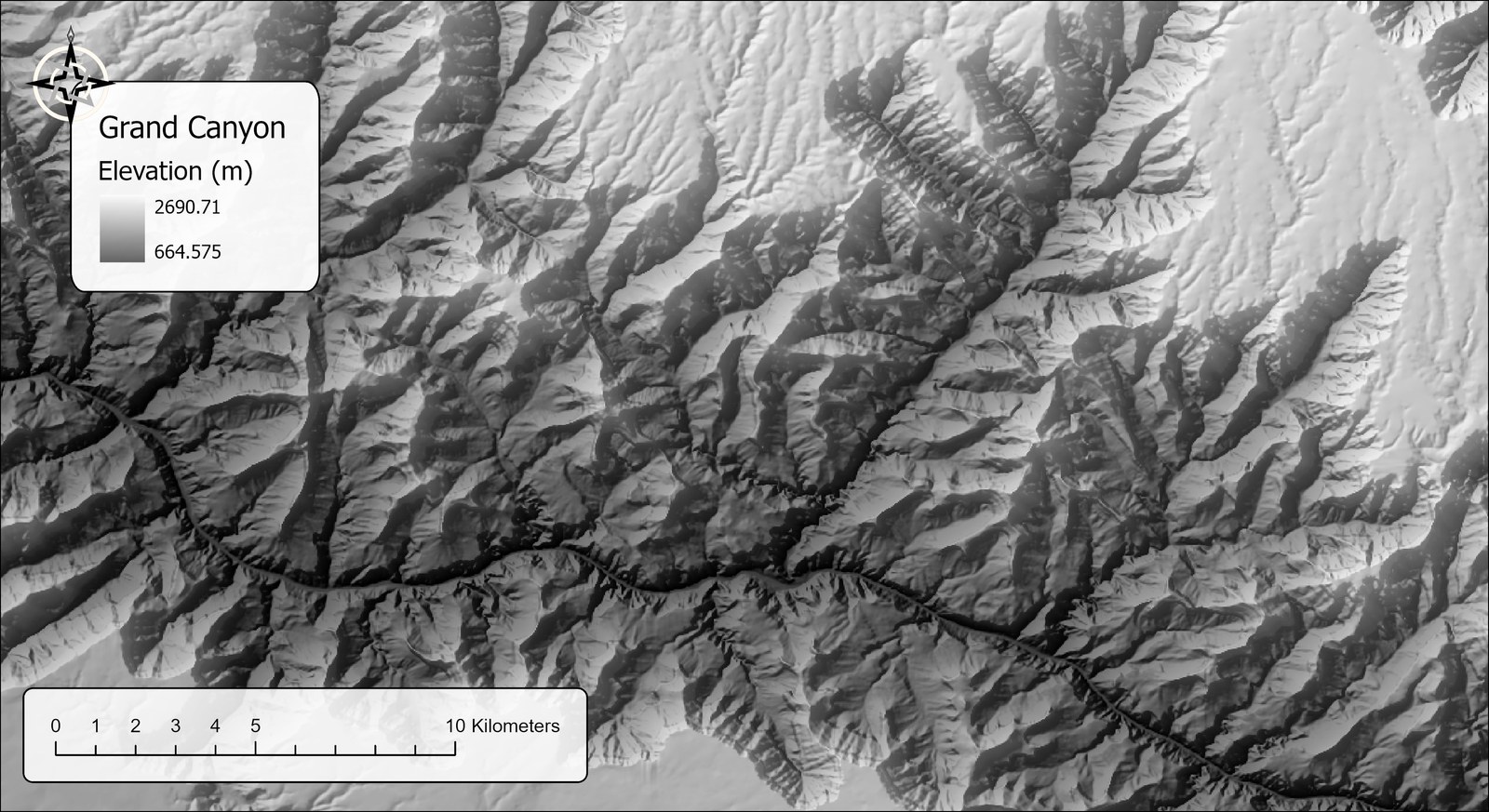
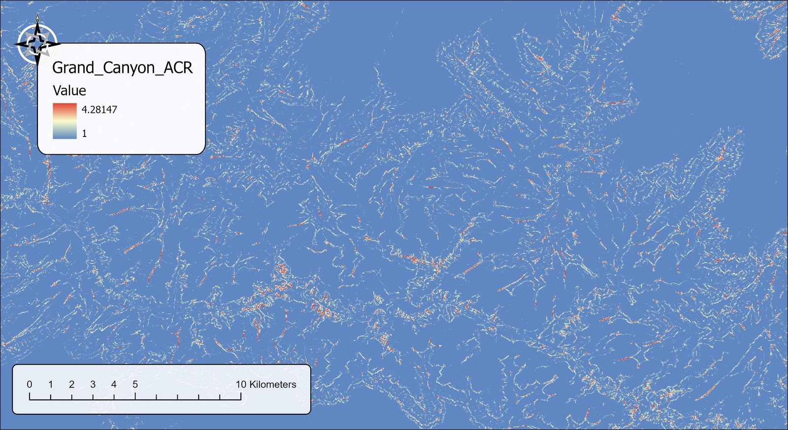
The example uses the same 30 m DEM of the Grand Canyon as the Surface Area and Ratio and Vector Ruggedness Measure pages, so the three measures can be compared on identical ground.
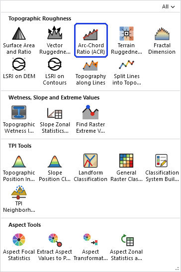
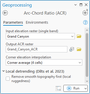
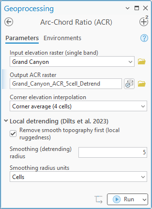
The dialog asks for the DEM, an output name (suggested from the input) and the corner interpolation method, with the detrending options in their own collapsible category. An Elevation units row appears only when the tool cannot work the units out for itself. There is no neighborhood radius, because ACR is inherently a 3 × 3 measure.
ACR beside the surface ratio
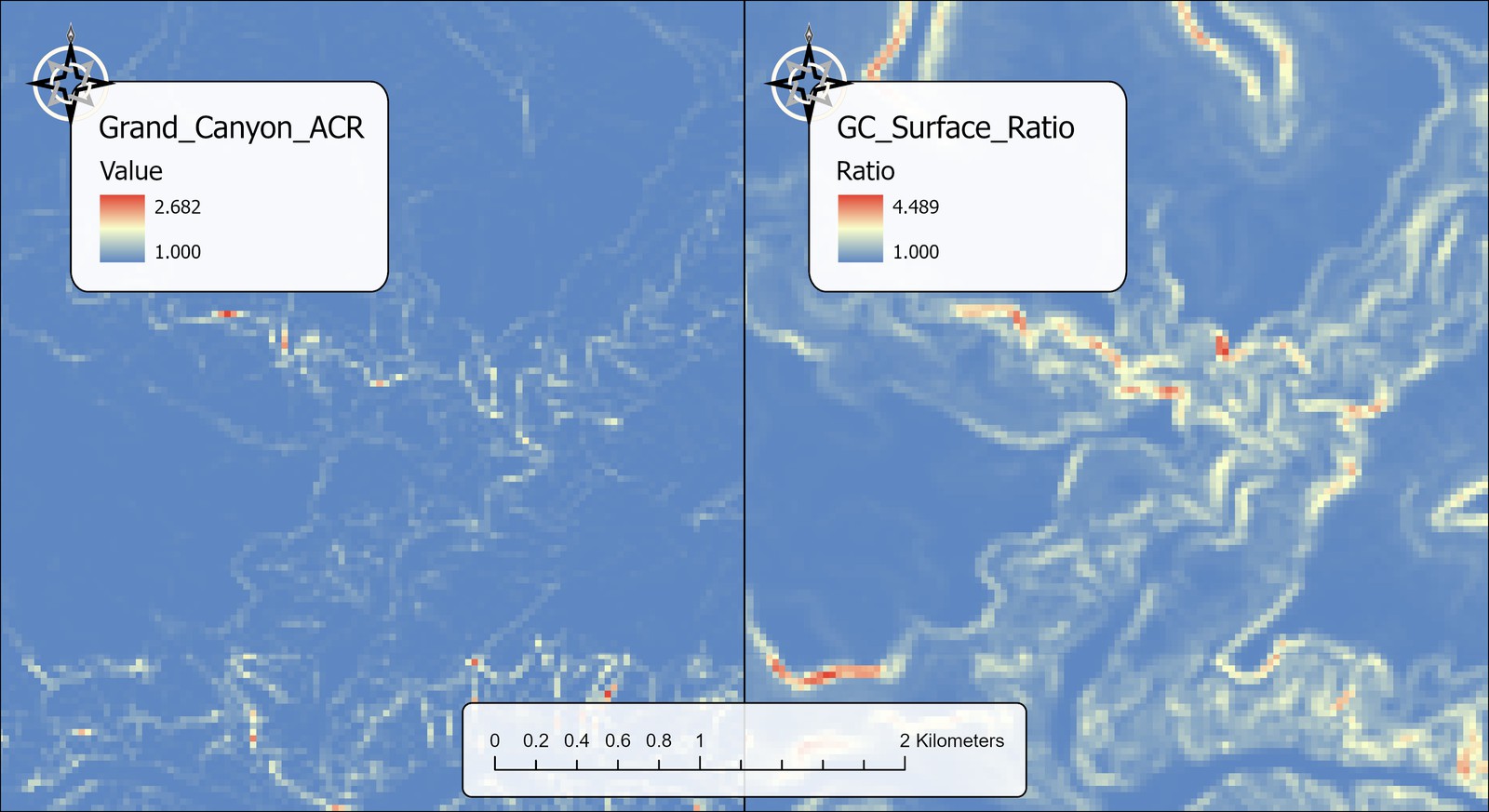
This pair is the whole argument for ACR in one picture. Every band on the right-hand map is real surface area, and if you want to know how much land there is, that is the map to use. But as a measure of roughness it is highly correlated with slope (a rank correlation of 0.99 across this DEM). It is a little better than slope for the purpose, because the eight triangles pass through the central cell and so catch the spikes and pits that a slope algorithm never sees, but most of what it shows is still steepness. Multiplying by the cosine of each cell's best-fit slope removes exactly that part, and what the left-hand map keeps is the part that a tilted plane cannot explain.
ACR-L with a 5-cell smoothing radius
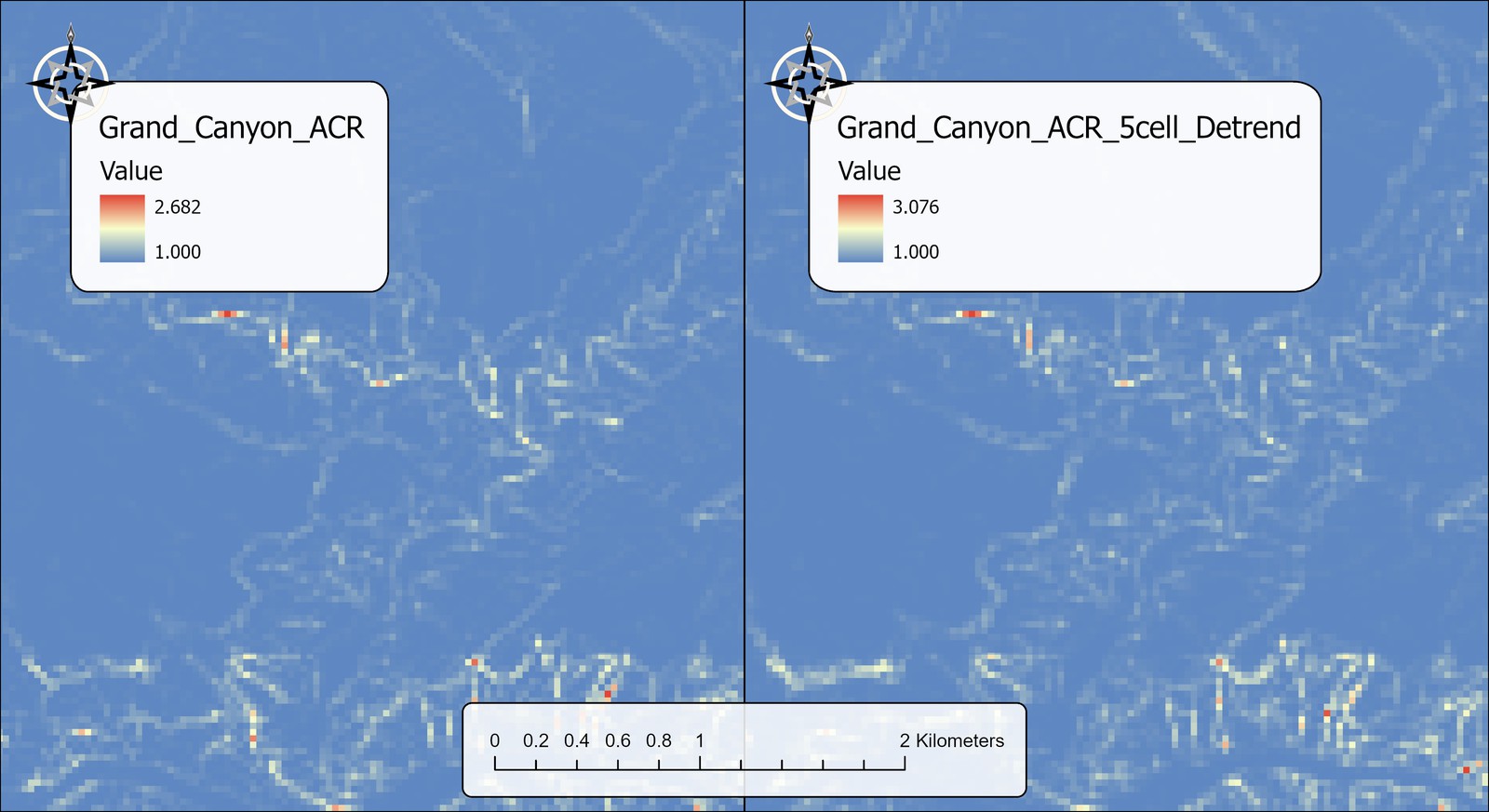
You might have expected detrending to lower the values, as it did for the surface ratio, so the higher maximum deserves an explanation. It follows directly from the difference between the two operations. Plain ACR measures roughness perpendicular to the local slope, so a ledge 10 m high on a 60° wall counts as only 5 m of relief square to the wall. Detrending with a 5-cell mean flattens that wall first: the broad tilt is subtracted away, the ledge is still 10 m high in the residual, and the residual's own local slope is much gentler than the wall's (across the canyon the mean slope falls from 24.7° to 14.3°), so ACR's cosine now discounts it far less. The steeper the ground, the bigger the difference:
| Slope of the original terrain | Mean ACR | Mean ACR-L (5 cells) |
|---|---|---|
| 0° to 10° | 1.003 | 1.002 |
| 10° to 25° | 1.016 | 1.016 |
| 25° to 40° | 1.020 | 1.027 |
| 40° to 55° | 1.036 | 1.071 |
| 55° and steeper | 1.066 | 1.166 |
On gentle ground the two are the same number. On the steepest ground ACR-L is about two and a half times as far above 1 as plain ACR, and across the whole DEM it is the larger of the two in 59% of cells. Neither is the correct one. Plain ACR asks how rough the wall is as a wall; ACR-L at 5 cells asks how much vertical relief there is at scales finer than 140 m, wherever it sits. Which of those your animal or your process responds to is the question to settle before choosing.
The output is a floating-point raster with a minimum of 1, carrying statistics, a histogram and bilinear pyramids so it draws correctly the moment it reaches the map, with a blue-yellow-red stretch applied by default. Outputs may go into a geodatabase or a folder; in a folder a name without an extension becomes a GeoTIFF.
The tool holds the whole DEM in memory at once, so the memory it needs grows with the number of cells. On most DEMs that is no concern. On a very large one the tool may need more memory than your computer has free, and then one of two things happens: Windows starts using the disk as overflow memory and the tool slows to a crawl, or the tool stops with an out-of-memory error. There is no fixed limit; it depends on how much memory your computer has free. If a DEM is too large, clip it to the area you need first.
Environment settings
The output matches the input DEM exactly: same extent, cell size and coordinate system. The Processing Extent, Snap Raster, Cell Size, Output Coordinate System and Mask environments are deliberately not applied, so that the delivered raster is the grid the ACR values were computed on; project, clip or resample the finished raster yourself if you need to. Pyramids are always built with bilinear resampling regardless of the Pyramid environment.
ModelBuilder
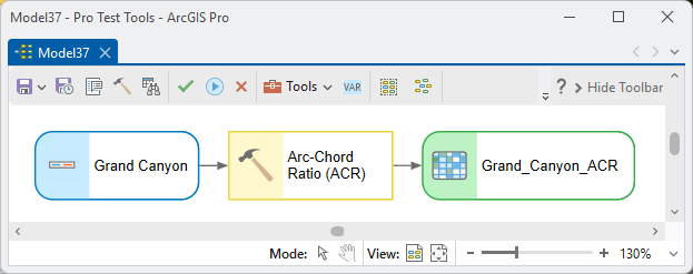
Parameters
| Label | Explanation | Data type |
|---|---|---|
| Input elevation raster (single band)Required · in_raster | The DEM. Must be single band; projected or geographic. Choose a layer from the map or browse to a dataset. | Raster Layer |
| Output ACR rasterRequired · out_raster | Floating point; 1 on flat or smoothly sloped terrain, higher where the surface is rough; NoData on the raster edge and wherever any cell of the 3 × 3 window is NoData. A name is suggested from the input. | Raster Dataset |
| Elevation unitsOptional · elev_units | Meters or Feet. Filled in and locked from the DEM's vertical coordinate system when it has one; geographic DEMs are assumed to be in meters; you are asked only when the DEM does not say. | String |
| Corner elevation interpolationRequired · corner_method | Diagonal midpoint (2 cells, original method) matches the 2004 paper and the legacy DEM Surface Tools (Jenness 2013); Corner average (4 cells) is the true bilinear estimate and the more accurate choice. Identical on planar slopes. Diagonal midpoint is the default; the dialog remembers the last choice made, as it does for the other options. | String |
| Remove smooth topography first (local ruggedness)Optional · detrend | Subtract a circular neighborhood mean of the DEM before computing, giving the local variant ACR-L of Dilts et al. (2023). Off by default. | Boolean |
| Smoothing (detrending) radiusOptional · detrend_radius | Radius of the smoothing mean. The default 1.5 cells is exactly a 3 × 3 mean; larger radii remove broader topography and so act as this tool's scale control. Used only when detrending is on. | Double |
| Smoothing radius unitsOptional · detrend_units | Cells, Meters, Kilometers, Feet or Miles; ground units are converted to cells from the cell size, per row on the spheroid for geographic DEMs, where the east–west radius is rounded to whole cells row by row. Used only when detrending is on. | String |
Python
import arcpy
arcpy.ImportToolbox(r"C:\path\to\JennessEnterprisesTools.pyt")  # your install path
# Standard ACR with the improved corner interpolation.
arcpy.jenness.ArcChordRatio(
    in_raster=r"C:\Project\Elev.gdb\DEM",
    out_raster=r"C:\Project\Elev.gdb\DEM_ACR",
    elev_units="Meters",
    corner_method="Corner average (4 cells)")
# The local (detrended) variant ACR-L, with a 3 x 3 smoothing mean.
arcpy.jenness.ArcChordRatio(
    in_raster=r"C:\Project\Elev.gdb\DEM",
    out_raster=r"C:\Project\Elev.gdb\DEM_ACRL",
    elev_units="Meters",
    corner_method="Corner average (4 cells)",
    detrend=True, detrend_radius=1.5, detrend_units="Cells")
Recommended citation
Credits and references
By Jeff Jenness, Jenness Enterprises (www.jennessent.com). The index is Du Preez's (2015); the contoured area is the eight-triangle surface area of Jenness (2004), which Du Preez cites for the raster case; the best-fit slope follows Horn (1981); and the local-detrending option and the three-generations framework follow Dilts et al. (2023).
- Dilts, T. E., M. E. Blum, K. T. Shoemaker, P. J. Weisberg, and K. M. Stewart. 2023. Improved topographic ruggedness indices more accurately model fine-scale ecological patterns. Landscape Ecology 38:1395–1410. doi.org/10.1007/s10980-023-01646-6
- Du Preez, C. 2015. A new arc-chord ratio (ACR) rugosity index for quantifying three-dimensional landscape structural complexity. Landscape Ecology 30:181–192. doi.org/10.1007/s10980-014-0118-8
- Horn, B. K. P. 1981. Hill shading and the reflectance map. Proceedings of the IEEE 69:14–47. doi.org/10.1109/PROC.1981.11918
- Jenness, J. S. 2004. Calculating landscape surface area from digital elevation models. Wildlife Society Bulletin 32:829–839. jennessent.com/downloads/WSB_32_3_Jenness.pdf; doi.org/10.2193/0091-7648(2004)032[0829:CLSAFD]2.0.CO;2
- Jenness, J. 2013. DEM Surface Tools for ArcGIS (v. 2.1.375). Jenness Enterprises. jennessent.com/arcgis/surface_area.htm
- Luckhurst, B. E., and K. Luckhurst. 1978. Analysis of the influence of substrate variables on coral reef fish communities. Marine Biology 49:317–323. doi.org/10.1007/BF00455026
- McCormick, M. I. 1994. Comparison of field methods for measuring surface topography and their associations with a tropical reef fish assemblage. Marine Ecology Progress Series 112:87–96. doi.org/10.3354/meps112087
- Risk, M. J. 1972. Fish diversity on a coral reef in the Virgin Islands. Atoll Research Bulletin 153:1–4. doi.org/10.5479/si.00775630.153.1
- Sappington, J. M., K. M. Longshore, and D. B. Thompson. 2007. Quantifying landscape ruggedness for animal habitat analysis: a case study using bighorn sheep in the Mojave Desert. Journal of Wildlife Management 71:1419–1426. doi.org/10.2193/2005-723
Licensing information
Works at every ArcGIS Pro license level (Basic, Standard, Advanced). No extension licenses are required; the surface areas and best-fit slopes are computed internally, without Spatial Analyst or 3D Analyst.
Related tools and pages
- About Topographic Roughness — choosing among the nine roughness measures, and the three generations of ruggedness index.
- Surface Area and Ratio — the contoured area and the flat-footprint ratio that ACR de-tilts.
- Vector Ruggedness Measure (VRM) — the other second-generation index, built on the same best-fit-plane normal.
- Terrain Ruggedness Index (TRI) — first-generation elevation-difference indices.
- Projecting Rasters — why this tool works on geographic DEMs directly.