

Topographic Position Index (TPI)
Summary
Computes the Topographic Position Index (TPI; Weiss 2001, after Guisan et al. 1999) of a DEM over a neighborhood: each cell's elevation minus the mean elevation of the cells around it. Positive values sit above their surroundings (ridges and hills), negative values sit below them (valleys and channels), and values near zero are flats and even mid-slopes. TPI is the raw ingredient behind the Slope Position Classification and Landform Classification tools, and it is useful on its own as a continuous measure of where a cell sits on the landscape.
The neighborhood is the scale of the analysis, and TPI is inherently scale-dependent: the same point can read as a valley at one scale and a hilltop at another, and both are valid. The neighborhood may be a circle or an annulus (the ring shape Weiss's own examples used), with the radius in cells or ground units, and it is computed exactly. The tool offers five outputs, any combination of which may be requested: raw TPI in the DEM's elevation units, TPI standardized in standard-deviation units at the neighborhood scale or at the DEM scale, TPI in percentile units, and an experimental TPI standardized by the neighborhood standard deviation of TPI. Three of these are the terrain-position metrics of Wilson and Gallant (2000). Everything is computed internally, with no Spatial Analyst extension.
The idea
The index is a difference: the elevation of a cell minus the mean elevation of a neighborhood around it.
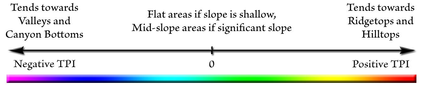
where z0 is the elevation of the cell and z̄ is the mean elevation of the cells in its neighborhood. The sign carries the meaning. A cell higher than the average of its surroundings has a positive index and tends toward a ridge or hilltop; a cell lower than its surroundings has a negative index and tends toward a valley or canyon bottom. A value near zero says only that the cell is close to the neighborhood mean, which happens both on flat ground and partway up a uniform slope; the slope of the cell tells those two cases apart, which is how the classification tools use it.
Five outputs
The dialog offers five output rasters. Any combination may be requested, and at least one is required. All five share the same neighborhood settings, and all are written as floating-point rasters with statistics, a histogram, metadata, and a diverging blue-to-white-to-red stretch from the raster's minimum to its maximum, blue toward the low end and red toward the high end.
1. TPI in elevation units
The raw index: the cell's elevation minus the neighborhood mean elevation, in the DEM's own vertical units.
This is absolute relief: a hill that stands 100 m above the average of its surroundings reads as roughly +100 wherever it occurs. It is Wilson and Gallant's (2000) “diff” (their equation 3.27) and the form Weiss (2001) computed, before he standardized it.
For example, +100 means the spot is about 100 m higher than the ground around it, and −20 means it sits about 20 m lower, in the same meters (or feet) as the DEM. The top of a 100 m hill reads close to +100 whether the hill rises from a plain or from the floor of a mountain valley, so a rule such as “at least 30 m above its surroundings” finds the same kind of feature everywhere on the map. It measures the climb, which is what an animal (or a person) on the ground actually faces.
2. TPI standardized at neighborhood scale
The raw index divided by the standard deviation of elevation within the cell's own neighborhood, in standard-deviation units. Where the neighborhood is perfectly flat, so that the standard deviation is zero, the output is zero.
where sz is the standard deviation of the neighborhood elevations. This makes the value relative to the variability of the cell's immediate surroundings, so the same relief reads differently in smooth and in rough terrain. It is Wilson and Gallant's “dev” (equation 3.30), and it is the form the bundled classification systems adapted from Weiss (2001) expect.
For example, stand on top of a 100 m hill. If the hill rises alone out of a flat plain, it is the only real bump for a long way around, and this output gives it a high value. Put an identical hill right next to it and the same summit gets a lower value, because the country around it is now hilly and the first hill no longer stands out as much. Same hill, same climb to the top; different score, depending on its company.
3. TPI in percentile units
For each cell, the number of neighborhood cells lower than the focal cell, as a percentage of the number of cells in the neighborhood.
A value near 0 means almost every neighbor is higher, so the cell is very low relative to its surroundings; a value near 100 means it is higher than nearly all of them. It is Wilson and Gallant's “pctl” (equation 3.31). This output takes much longer to compute than the others, because every cell must be compared with every one of its neighbors, and the time grows with the size of the neighborhood.
For example, the top of a 100 m hill on a plain is higher than nearly everything around it, so it scores close to 100. So does the top of a 3 m rise on the same plain, and so does a mountain summit. This output only asks “is this spot higher or lower than most of the ground around it?”, not “by how much?” It is good at finding the local high spots and low spots in any country, flat or rugged, but it cannot tell a small rise from a major ridge.
4. TPI standardized at DEM scale
The cell's elevation standardized over the whole raster: the elevation minus the mean elevation of the entire DEM, divided by the standard deviation of the entire DEM.
This output is independent of the neighborhood. It expresses how high or low a cell sits within the elevation distribution of the whole DEM, so it tracks absolute elevation rather than position relative to the surroundings, and it is likely the least used of the five. It is offered here for completeness; the classification tools do not compute it on the fly, though a raster of it may be supplied to them as an existing input.
For example, on a map that runs from a low river valley up into high mountains, the top of a 100 m hill on the valley floor can come out negative, because it is still lower than most of the map, while a flat meadow high in the mountains comes out strongly positive. This output tells you how high a place is compared with the whole map, not whether it is a hill, and its values change if the map is cut to a different area.
5. TPI standardized by the neighborhood standard deviation of TPI (experimental)
The raw index divided by the standard deviation of the raw index itself within the cell's neighborhood, in standard-deviation units. Where the neighborhood TPI is uniform, the output is zero.
The TPI standardized at neighborhood scale divides by the spread of the elevations in the neighborhood; this output divides by the spread of the TPI values there. The difference matters on a long uniform slope. The elevations in such a neighborhood vary a great deal, because the ground rises steadily across it, so the neighborhood-standardized TPI is damped by the regional slope; the TPI values there vary very little, because every cell is close to its neighborhood mean, so this output measures a cell's position against the local roughness of the terrain-position surface rather than against the local relief. That is also its weakness. On a smooth or planar slope both the numerator and the denominator approach zero, and the quotient amplifies whatever noise is in the DEM. For that reason it is offered only here, for exploration, and the Slope Position Classification and Landform Classification tools do not offer it when they compute TPI on the fly, where the neighborhood-standardized TPI behaves well in the same places. Supplied to them as an existing raster, it is treated as a TPI in standard-deviation units and classified without a warning, so use it that way only deliberately. It is not part of Wilson and Gallant (2000).
For example, a 100 m hill standing on a long, even hillside stands out strongly here, because nothing else nearby breaks the slope. The same hill in broken country full of knolls and gullies scores lower, because bumps are common there. This output asks whether a feature is unusual for its own patch of ground. On smooth, featureless ground, though, tiny bumps in the DEM can get large values, so the map can look speckled in exactly the places where there is nothing to see on the ground.
Raw or standardized?
Raw TPI keeps its meaning across a landscape: a threshold of +10 m picks out the same amount of relief everywhere, which is usually what an ecological question needs, because an animal experiences the actual height of a ridge and not its height relative to the local variability. Dickson and Beier (2007) used raw thresholds of this kind in their study of cougar movement. Standardized TPI, Weiss's (2001) choice, makes a cell's value relative to the variability around it, so a cell must stand further above its surroundings to count as a ridge where the terrain is rough than where it is smooth, and a small rise on a plain and a large hill in the mountains can receive the same value. That adapts a classification to each landscape and makes very different terrains comparable, but it can mislead if it is not what you expect. The classification systems record which form their thresholds assume, and the classification tools warn when a raster of a different kind is supplied. The warning tells apart only three kinds, raw, standard-deviation and percentile: the DEM-scale and experimental outputs both count as standard-deviation kinds, so they pass a system written for the neighborhood-standardized TPI without a warning.
The neighborhood and its scale
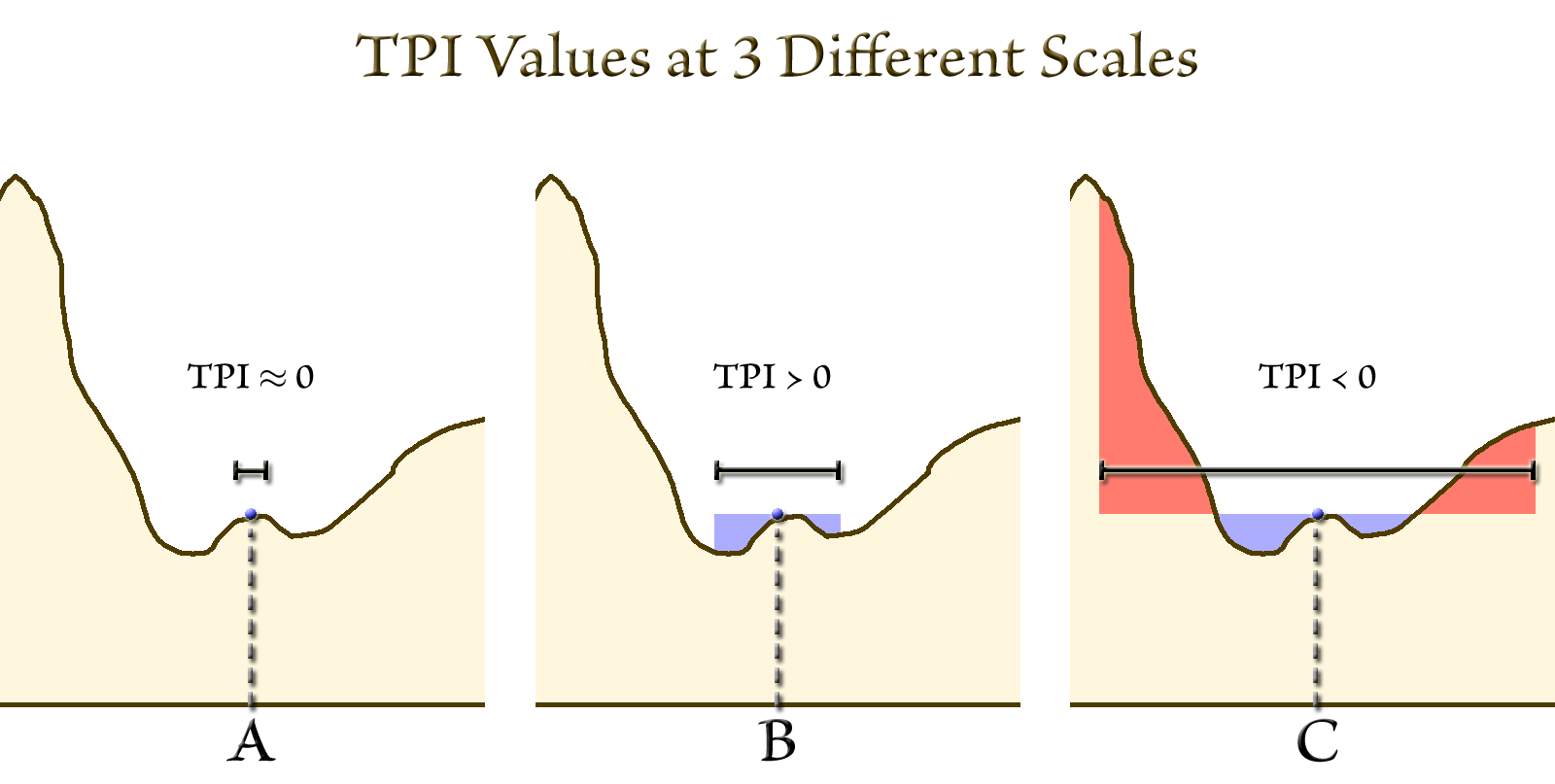
The neighborhood defines which cells are “around” a cell, and its size is the scale of the analysis. The same point on a small hill inside a larger valley has an index near zero when the neighborhood is smaller than the hill, a strongly positive index when the neighborhood takes in the whole hill, and a negative index when it reaches the valley walls on either side. Each of those answers is correct at its own scale.
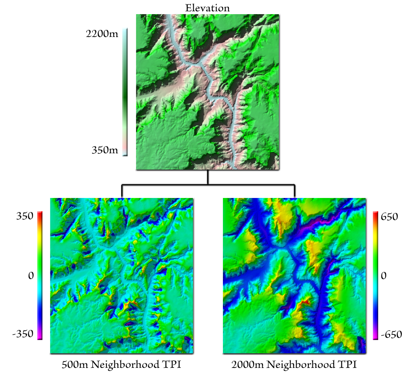
A small neighborhood picks out small, local hills and hollows; a large one picks out broad ridges and valleys. Choose the scale that matters for the question. A wide-ranging animal responds to the major ridgelines around it rather than to minor bumps underfoot, so a larger neighborhood suits it; a question about soil moisture or a small drainage wants a smaller one. The two maps below were computed from the same DEM with circular neighborhoods of 500 m and 2,000 m radius. The smaller neighborhood finds the extremes in the side drainages of the canyon; the larger one highlights the whole canyon system. The range of the index also grows with the neighborhood, from about ±350 m at 500 m to about ±650 m at 2,000 m, because a bigger neighborhood spans more relief.
The neighborhood may be a circle, every cell whose center lies within the radius, or an annulus, the ring between an inner and an outer radius. Weiss's own examples used annuli: on a 30 m DEM, an inner radius of 5 cells and an outer radius of 10 for his fine-scale index, and 62 and 67 cells for his coarse-scale index, which he named tpi300 and tpi2000 after their outer radii in meters. An annulus ignores the cells nearest the focal cell and compares it with a band of terrain at a chosen distance. The radius may be given in cells or in ground units (meters, kilometers, feet or miles); a ground-unit radius is converted to cells using the DEM's cell size.
The neighborhoods are computed exactly from the cell geometry, so they avoid the cell-rounding quirks that some focal-statistics tools show with circles and annuli, and NoData cells are left out of the neighborhood mean and standard deviation rather than poisoning them. On a geographic (latitude/longitude) DEM a ground-unit radius is worked out separately for the east-west and north-south directions: the east-west width of a cell in meters is computed for every row on the spheroid and shrinks toward the poles, while the north-south height is nearly constant, so the neighborhood is an ellipse in pixel space that is a circle on the ground, recomputed row by row. For the mean and standard deviation the east-west radius is rounded to a whole number of cells for each band of rows, so the circle is exact to within about half a cell east-west; the percentile uses the exact radius.
The neighborhood is the one setting worth trying several ways before a full run, and the TPI Neighborhood Sampler is built for that. It takes a snapshot of the DEM inside the map view and repaints the TPI as a slider moves through the radii, with a second slider for a classification threshold and a pin that plots one cell's TPI against the radius. The radius, its units and the TPI type it settles on are this tool's own parameters, and its Copy Settings button writes the matching call.
A tour of the dialog
The examples use the 30 m Grand Canyon DEM, with a circular neighborhood of 500 m, the same radius as the left half of the two-neighborhood figure above.
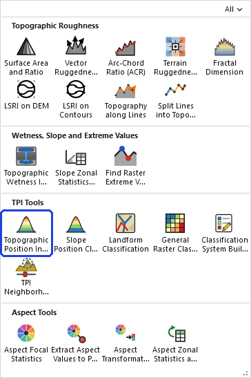
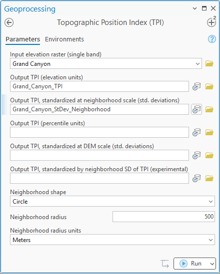
The dialog asks for the DEM, then lists the five outputs in the order described above. Each is optional, and clearing an output's name skips it; when a DEM is chosen, a name for the raw TPI is suggested from it. Below the outputs come the neighborhood shape, its radius, the inner radius, and the radius units, followed by the DEM's elevation units. The inner radius applies only to an annulus, and the elevation units are detected when the DEM carries a vertical coordinate system and asked for only when it does not, so with a circle and this DEM neither row appears. The elevation units label the raw output only; they do not change any of the values.
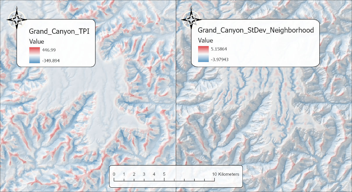
The two maps show the difference between measuring the climb and measuring how much a spot stands out from its own surroundings. In the raw TPI on the left, the top of the plateau is nearly white: its gentle swells are lost on a color scale that has to stretch from −350 to +447 m to cover the side canyons, and only the rims and drainages show color. In the standardized TPI on the right, the plateau top is full of small ridges and swales, because in that quiet country a little relief is a lot compared with everything else in the neighborhood, while the canyon walls, where big relief is everywhere, are toned down. Neither version needs more topography than the other to show a feature; they need different surroundings. A feature stands out in the raw TPI when it is tall, and in the standardized TPI when it is unusual for its neighborhood, which on a quiet plateau can mean only a modest rise or dip.
Every output arrives with a diverging stretch from its minimum to its maximum: blue at the low end, white at the middle of the range, red at the high end. The middle of the range is near zero only when the raster's lows and highs are of similar size, so read the legend rather than assuming white means zero. Each output's metadata records the DEM it came from, the neighborhood, and two marks that the classification tools read back. One names the kind of TPI in the raster (raw, neighborhood-standardized, DEM-standardized, percentile, or the experimental TPI-standardized form), so that Slope Position Classification and Landform Classification can warn when a supplied raster does not match the units a classification system expects. The other records the outer radius of the neighborhood, so that the Landform tool can warn when the rasters given as its small- and large-neighborhood inputs appear to be swapped or to have the same radius. The DEM-scale output carries the type mark but no radius mark, since no neighborhood went into it.
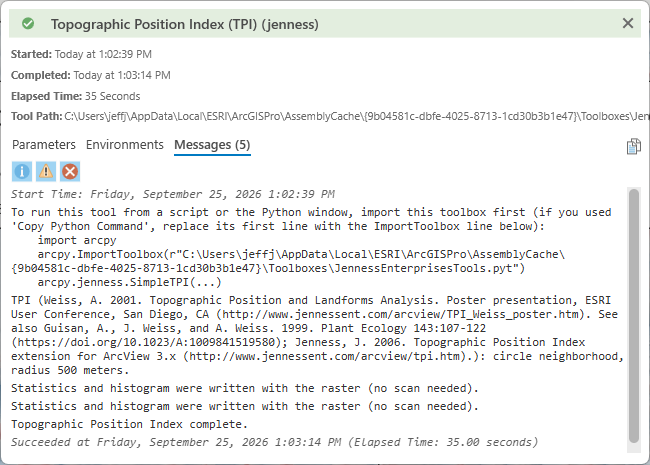
The tool holds the whole DEM in memory at once, so the memory it needs grows with the number of cells. On most DEMs that is no concern. On a very large one the tool may need more memory than your computer has free, and then one of two things happens: Windows starts using the disk as overflow memory and the tool slows to a crawl, or the tool stops with an out-of-memory error. There is no fixed limit; it depends on how much memory your computer has free. If a DEM is too large, clip it to the area you need first.
ModelBuilder
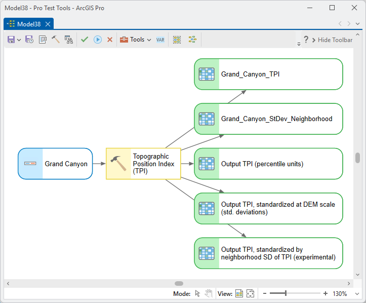
Parameters
| Label | Explanation | Data type |
|---|---|---|
| Input elevation raster (single band)Required · in_raster | The DEM, single band. Projected and geographic (latitude/longitude) coordinate systems are both supported; on a geographic DEM a ground-unit radius is sized per row on the spheroid so the neighborhood stays a true circle on the ground. | Raster Layer; Raster Dataset |
| Output TPI (elevation units)Optional · out_tpi | The raw TPI: each cell's elevation minus the mean elevation of its neighborhood, in the DEM's elevation units. A name is suggested from the input. Leave any output blank to skip it; at least one of the five outputs is required. | Raster Dataset |
| Output TPI, standardized at neighborhood scale (std. deviations)Optional · out_dev | The raw TPI divided by the standard deviation of elevation within each cell's neighborhood, in standard-deviation units; 0 where the neighborhood is flat. | Raster Dataset |
| Output TPI (percentile units)Optional · out_pctl | The count of neighborhood cells lower than the focal cell as a percentage of the number of cells in the neighborhood, from 0 for the lowest cell. The cell itself is counted in a circle, so the highest cell scores 100(n − 1)/n for n cells (an annulus excludes the cell, and its highest scores 100). The tool reports the highest possible value for the neighborhood in its messages, and the classification tools warn whenever a percentile class threshold cannot be reached with the neighborhood used. Much slower than the other outputs, and slower still as the neighborhood grows. | Raster Dataset |
| Output TPI, standardized at DEM scale (std. deviations)Optional · out_demstd | The elevation standardized over the whole raster: the elevation minus the DEM's mean elevation, divided by the DEM's standard deviation. Independent of the neighborhood. | Raster Dataset |
| Output TPI, standardized by neighborhood SD of TPI (experimental)Optional · out_devtpi | The raw TPI divided by the standard deviation of the raw TPI within each cell's neighborhood; 0 where the neighborhood TPI is uniform. Numerically unstable on smooth or planar slopes. The classification tools do not offer it on the fly, and treat it as a standard-deviation TPI if it is supplied as an existing raster. | Raster Dataset |
| Neighborhood shapeRequired · nb_shape | Circle (all cells within the radius) or Annulus (a ring between an inner and an outer radius). Default Circle. | String |
| Neighborhood radiusRequired · nb_outer | The radius, or for an annulus the outer radius, in the units chosen below. This sets the spatial scale of the analysis; larger radii capture broader landforms. Default 10. | Double |
| Neighborhood inner radius (annulus only)Optional · nb_inner | For an annulus, the inner radius of the ring; cells nearer than this are excluded. Ignored for a circle. Default 0. | Double |
| Neighborhood radius unitsRequired · nb_units | Cells, or a ground unit: Meters, Kilometers, Feet or Miles. A ground-unit radius is converted to cells from the DEM's cell size; on a geographic DEM it is converted separately on each axis and per row, so the neighborhood is a true circle on the ground. Default Cells. | String |
| Elevation unitsOptional · elev_units | Meters or Feet. Detected and locked when the DEM defines a vertical coordinate system. Used only to label the raw TPI output; it does not change any value. | String |
Python
Import the toolbox once, then call the tool with keyword arguments. The comment block lists every valid choice for the list-driven parameters; pass those strings exactly as shown.
import arcpy
arcpy.ImportToolbox(r"C:\path\to\JennessEnterprisesTools.pyt")  # your install path

# ---- valid options for the list-driven parameters ------------------------
# nb_shape:   "Circle" | "Annulus"
# nb_units:   "Cells" | "Meters" | "Kilometers" | "Feet" | "Miles"
# elev_units: "Meters" | "Feet"
# outputs (all optional; any combination, at least one):
#   out_tpi     raw TPI (elevation units)
#   out_dev     TPI standardized at neighborhood scale (std. deviations)
#   out_pctl    TPI in percentile units (slow on large neighborhoods)
#   out_demstd  TPI standardized at DEM scale (std. deviations)
#   out_devtpi  TPI / neighborhood SD of TPI (experimental)

# Raw and neighborhood-standardized TPI over a 300 m annulus
arcpy.jenness.SimpleTPI(
    in_raster=r"D:\Project\Elev.gdb\DEM",
    out_tpi=r"D:\Project\Elev.gdb\DEM_TPI",
    out_dev=r"D:\Project\Elev.gdb\DEM_TPI_dev",
    nb_shape="Annulus", nb_outer=300, nb_inner=100, nb_units="Meters",
    elev_units="Meters")

# Raw TPI only, over a 10-cell circle
arcpy.jenness.SimpleTPI(
    in_raster=r"D:\Project\Elev.gdb\DEM",
    out_tpi=r"D:\Project\Elev.gdb\DEM_TPI_10",
    nb_shape="Circle", nb_outer=10, nb_units="Cells")
Recommended citation
Credits and references
By Jeff Jenness, Jenness Enterprises (www.jennessent.com), modernizing his Topographic Position Index extension for ArcView 3.x (Jenness 2006), which automated the methods of Andrew Weiss's 2001 poster. The manual figures on this page are from that extension.
- Dickson, B. G., and P. Beier. 2007. Quantifying the influence of topographic position on cougar (Puma concolor) movement in southern California, USA. Journal of Zoology 271:270–277. doi.org/10.1111/j.1469-7998.2006.00215.x
- Guisan, A., S. B. Weiss, and A. D. Weiss. 1999. GLM versus CCA spatial modeling of plant species distribution. Plant Ecology 143:107–122. doi.org/10.1023/A:1009841519580
- Jenness, J. 2006. Topographic Position Index (tpi_jen.avx) extension for ArcView 3.x, v. 1.3a. Jenness Enterprises. jennessent.com/arcview/tpi.htm
- Weiss, A. 2001. Topographic Position and Landforms Analysis. Poster presentation, ESRI User Conference, San Diego, CA. jennessent.com/arcview/TPI_Weiss_poster.htm
- Wilson, J. P., and J. C. Gallant. 2000. Terrain analysis: principles and applications. John Wiley and Sons, New York. (Equations 3.27, 3.30 and 3.31.)
Licensing information
Works at every ArcGIS Pro license level (Basic, Standard, Advanced). No extension licenses are required; the neighborhood statistics are computed internally, without Spatial Analyst.
Related tools and pages
- About TPI — the index, scale, and the classifications built on it.
- Slope Position Classification — slope-position classes from one TPI plus slope.
- Landform Classification — landform classes from TPI at two scales plus slope.
- General Raster Classification — the same classification systems applied to any raster.
- Classification System Builder — author the systems those tools apply.
- About Topographic Roughness — how topographic position relates to the roughness measures, and why scale matters for both.
- Projecting Rasters — project the DEM with bilinear interpolation before deriving TPI.
- TPI Neighborhood Sampler — try neighborhood sizes and thresholds on a snapshot of the DEM, with sliders, before running the tools.