

Topography along Lines
Summary
Adds attribute fields describing the topography along each line of a polyline feature class: how long the line is on the ground versus on the map, how much of it climbs and descends, how steep and how variable its slopes are, which way it heads and how consistently, how much it meanders, and how convoluted its path is. Elevation comes from the polylines' own Z values or is sampled from a DEM by bilinear interpolation; each line is reduced to short straight three-dimensional segments, and every one of the 36 available statistics is computed from those segments. You choose which statistics to compute and which field each one is written to, much as in the Calculate Geometry Attributes tool, and the fields are written into the input feature class. No Spatial Analyst or 3D Analyst license is needed.
Why measure the route instead of the landscape
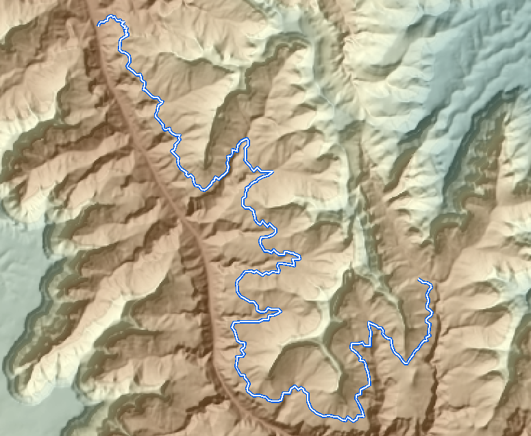
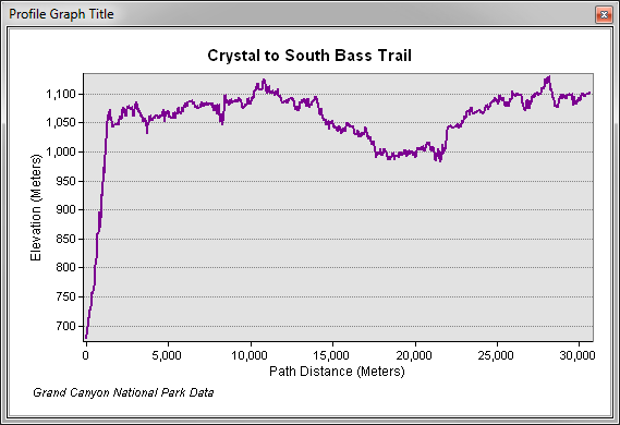
The raster tools in this menu describe the landscape, cell by cell. But if your question is about movement, what an animal (or hiker!) actually experiences is the route they take, and a route can be gentle through terrain that is anything but. The trail above crosses the Grand Canyon, and after its first kilometer it stays between about 990 and 1,130 m for the next thirty. A raster roughness index would tell you the canyon is rough; it would tell you nothing about how hard the trail is. This tool answers the second question. It works for anything you can represent as a line: GPS tracks and movement paths, trails and roads, transects, stream centerlines, fence lines, proposed corridors and skid trails. One caution for a GPS track: the straight line between two fixes is only a guess at the route the animal took, so sampling the DEM every cell along it describes ground the animal may never have crossed. The whole-track statistics are still a fair summary of that assumed route; for questions about the individual steps, the At the vertices only mode of Split Lines into Topography Segments, which measures each step as one feature, is the better fit. For each line it samples the elevation along the route, breaks the route into straight three-dimensional pieces, and reduces those pieces to whichever of the 36 statistics you ask for.
Direction of travel
This is the one convention you must keep in mind, so I will state it first. Many of these statistics depend on which way the line goes. A line that climbs 100 m from west to east descends 100 m from east to west: its uphill and downhill lengths swap, its elevation gain and loss swap, and its mean direction flips by 180°. Every direction-dependent statistic (cumulative elevation gain and loss, net elevation change, the uphill and downhill lengths and proportions, and mean direction) describes the line traveling in the direction of its geometry, from its first vertex to its last. That is the order the vertices were digitized in, or the order the GPS fixes were recorded in, and it is not necessarily the direction the animal or the hiker went. If you need the statistics the other way, reverse the line first with the Flip Line geoprocessing tool, and run the tool again. The direction-independent statistics (the lengths, surface ratio, slope statistics, sinuosity, fractal dimension, total curvature, reversal count, and every measure of directional spread) come out the same either way, and the metadata of each direction-dependent field created says that reversing the line reverses its value.
The segment model
Everything the tool reports comes from one construction: each line is reduced to a chain of straight segments, each with an X, Y and Z at both ends. How those segments are made depends on where the elevation comes from.
Z values from the polylines. If the feature class is Z-enabled (a PolylineZ from a GPS unit, a 3D digitizing session, or the companion Split Lines into Topography Segments tool), you may use its own vertex elevations, in which case each existing vertex is a segment end and nothing is added between them. The statistics then describe the line exactly as it was recorded, at whatever spacing the vertices have.
Elevation sampled from a DEM. Otherwise, or by choice, the tool samples a DEM. It places sample points along each line at a regular ground interval equal to the smaller of the DEM's cell width and cell height, and it always keeps every original vertex as well as the first and last point of every part, so real bends stay where they were digitized rather than being rounded across. Each vertex-to-vertex leg is cut into the fewest equal pieces that are no longer than the interval. On a 30 m DEM, a straight line 300 m long becomes ten 30 m segments; a 45 m leg to a corner becomes two segments of 22.5 m, and a 61 m leg three of 20.3 m. Each sample point is projected into the DEM's own coordinate system and its elevation is found by bilinear interpolation from the four surrounding cell centers. The DEM itself is never projected; projecting a raster resamples and degrades it, so the points go to the raster rather than the raster to the points (see Projecting Rasters). A sample point that falls on NoData, or outside the DEM, breaks the chain: the segments touching it are dropped, and the valid runs on either side of the gap are treated as separate pieces of the line, exactly like the parts of a multipart line. No turn angle, reversal, sinuosity chord or fractal path ever spans a gap, the first sample after a gap starts the next piece, and the tool reports how many segments were dropped and at how many gaps the chain was broken.
Different datums. When the polylines and the DEM are on different datums, the sample points are moved onto the DEM's datum with a geographic transformation before its elevations are read: the one named in the Geographic Transformations environment when it applies, otherwise Esri's recommended transformation for the pair. The tool names the transformation it used in its messages and warns in the dialog as soon as it sees the datums differ. The lines themselves are never moved.
Segment lengths. Each segment's planimetric length is the geodesic distance between its ends, measured on the spheroid, so it is correct whether the data are projected or in latitude and longitude. Its surface length is the true three-dimensional distance, the hypotenuse of the planimetric length and the elevation change:
with the elevation change converted into the same unit as the planimetric length first, so that the two legs of the triangle agree. On a 30 m DEM whose surface rises 3 m across a cell, a segment has a planimetric length of 30 m and a surface length of √(30² + 3²) = 30.15 m; the same segment on flat ground is exactly 30 m both ways. That small difference, summed over a whole line, is what separates the map length of a route from the distance actually walked.
Multipart lines. A line made of several disconnected pieces is handled piece by piece. The first and last vertex of every piece are included, and no segment is ever built across the gap between pieces, so a gap never counts as a climb, a descent or a turn.
The statistics
All 36 are listed here by kind; the dialog offers them as a single list in its own order. Where a formula matters I give it, and I follow each group with the numbers for one simple example: a straight line running due east for 300 m across a 30 m DEM that rises steadily 1 m for every 10 m eastward, so that every one of its ten segments is 30 m long on the map and climbs 3 m.
Lengths
| Statistic | Definition | Units |
|---|---|---|
| Planimetric Length (geodesic) | The sum of the segments' horizontal lengths: the length of the line on the map, measured on the spheroid. | Length unit |
| Surface Length (geodesic) | The sum of the segments' three-dimensional lengths: the distance actually traveled over the ground. | Length unit |
| Surface Ratio | Surface length divided by planimetric length. Exactly 1 on flat ground, larger over rough or steep terrain; the line-based cousin of the surface ratio in Surface Area and Ratio. | Unitless |
For the example line: ten segments of 30.15 m give a surface length of 301.5 m against a planimetric length of 300 m, and a surface ratio of 1.005. (In a real run the planimetric length comes out 300.08 m rather than 300, the difference between a geodesic distance on the spheroid and a planar distance on the projection, and those extra 8 cm tip the line past ten intervals, so it is cut into eleven equal segments of 27.28 m rather than ten of 30 m. On a uniform grade the totals come out the same.)
Uphill, downhill and flat
| Statistic | Definition | Units |
|---|---|---|
| Length Uphill, Length Downhill, Length Perfectly Flat | The summed surface lengths of the segments that climb, descend, or have exactly zero elevation change, in the direction of travel. | Length unit |
| Proportion Uphill, Proportion Downhill, Proportion Perfectly Flat | Each of those lengths divided by the total surface length. The three sum to 1. | Unitless |
Perfectly flat means exactly zero change between two sampled elevations. Exactly zero change between two interpolated elevations is rare on natural terrain. For the example line, all 301.5 m are uphill, so Proportion Uphill is 1 and the other two are 0; traverse it the other way and all of it is downhill.
Elevation
| Statistic | Definition | Units |
|---|---|---|
| Cumulative Elevation Gain | The sum of every segment's rise, ignoring the falls: the total climbing. | Elevation units |
| Cumulative Elevation Loss | The sum of every segment's fall, as a positive number: the total descending. | Elevation units |
| Net Elevation Change | Gain minus loss: the elevation of the last vertex minus the first, when the chain is unbroken. Otherwise the sum of all such net elevation changes in the multiple pieces of a multipart polyline, or of a line broken by a NoData gap. | Elevation units |
| Total Vertical Relief Traveled | Gain plus loss: all the climbing and all the descending together. | Elevation units |
| Minimum Elevation, Maximum Elevation, Elevation Range | The lowest and highest sampled elevation along the line, and their difference. | Elevation units |
| Minimum Elevation X / Y, Maximum Elevation X / Y | The coordinates of the lowest and highest sampled point, reported in the polyline dataset's own coordinate system even when the DEM is in another one. If the extreme elevation occurs at more than one sampled point, the first one along the line is reported. | Coordinate units |
| Reversal Count | How many times the line switches between climbing and descending, counted within each part; perfectly flat segments are skipped rather than counted as a switch. | Count |
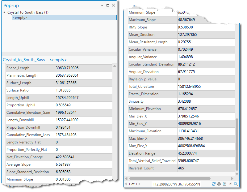
For the example line: gain 30 m, loss 0, net change +30 m, relief traveled 30 m, range 30 m, and no reversals. The Grand Canyon trail in the profile above is the interesting contrast: its net change is 423 m, while its total vertical relief traveled adds every one of those small climbs and descents, which is the quantity a net figure hides.
Slope
| Statistic | Definition | Units |
|---|---|---|
| Average Slope | The mean of the segments' absolute slopes, each weighted by its surface length, so a long steep pitch counts for more than a short one. | Slope unit |
| Minimum Slope, Maximum Slope | The shallowest and steepest segment slopes. Both are absolute steepness: a segment falling at 20° and one rising at 20° have the same slope. | Slope unit |
| Slope Standard Deviation | The surface-length-weighted standard deviation of the segment slopes: how variable the steepness is along the line. | Degrees, always |
| RMS Slope | The surface-length-weighted root mean square of the segment slopes, a measure that emphasizes the steep pitches more than the plain average does. | Degrees, always |
Every segment's slope is the angle whose tangent is its elevation change over its planimetric length, and all slope arithmetic is done in degrees. Only at the end are Average, Minimum and Maximum Slope converted to percent if you asked for percent (percent = 100 × tan of the angle, with the angle in radians: every trigonometric function in ArcGIS Pro, in the Raster Calculator, the Spatial Analyst Tan tool, the Field Calculator and Arcade, takes radians, so multiply degrees by π/180 before applying it). The reason is that the mean of percent slopes is not the true mean slope. Take two equal segments at 10° and 60°: the mean angle is 35°, which is a 70% slope. But 10° is 17.6% and 60° is 173.2%, whose mean is 95.4%, which converts back to 43.7°, a very different answer. Averaging angles gives the right answer; averaging percentages does not, because the tangent function grows faster and faster as slopes steepen. The standard deviation and RMS have no exact conversion from degrees to percent at all, so they are always reported in degrees regardless of the slope unit. For the example line every segment has the same slope, arctan(3/30) = 5.71°, which is a 10% slope; the average, minimum and maximum are all 5.71° (or 10%), and the standard deviation is 0.
Direction
These statistics treat every segment as a vector whose length is the segment's surface length and whose direction is its compass bearing, measured clockwise from north. Sum the vectors and you get a resultant; how long that resultant is, compared with the total length of the segments, tells you how consistently the line heads one way. These are the standard circular statistics; About Aspect explains them with more room, and Aspect Zonal Statistics as Table computes the same set for the cells of an aspect raster. The picture is easiest with four equal steps.
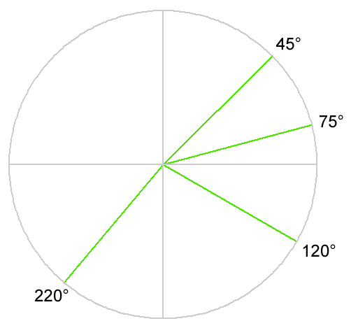
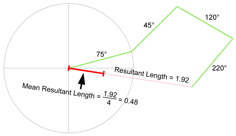
In the tool, each segment i has surface length Li and bearing θi, and the sums are weighted by length:
For the four equal steps, S = 1.896 and C = −0.300, so the resultant is √(1.896² + 0.300²) = 1.92 and the mean resultant length is 1.92 / 4 = 0.48, exactly as in the figure. The mean direction is the bearing of that resultant, atan2(S, C) = 99°, a little south of east.
| Statistic | Definition | Units |
|---|---|---|
| Mean Direction | The bearing of the resultant, atan2(S, C), as a compass azimuth. Direction-dependent: reversing the line adds 180°. | Degrees (azimuth) |
| Mean Resultant Length | R̄ itself, from 0 to 1. A value of 1 means every segment points the same way (a straight line); a value near 0 means the headings cancel out. | Unitless |
| Circular Variance | 1 − R̄ (Mardia and Jupp 2000; Fisher 1993). 0 for a straight line, up to 1. | Unitless |
| Angular Variance | 2(1 − R̄) (Batschelet 1981). 0 up to 2. | Unitless |
| Circular Standard Deviation | √(−2 ln R̄) (Mardia and Jupp; Fisher), converted from radians to degrees. Undefined when R̄ = 0. | Degrees |
| Angular Deviation | √(2(1 − R̄)) (Batschelet), converted to degrees; it tops out at 81.03°. | Degrees |
| Rayleigh p-value | The Rayleigh test of whether the line has a preferred direction at all, calculated with equation 27.4 of Zar (1999) and using the segment count as the sample size. A small p-value means the headings are not uniformly scattered. | Unitless |
For the four steps, R̄ = 0.48 gives a circular variance of 0.52, an angular variance of 1.04, a circular standard deviation of √(−2 ln 0.48) = 1.21 radians = 69.4°, an angular deviation of √(2 × 0.52) = 1.02 radians = 58.4°, and a Rayleigh p-value of 0.42, which is to say that four steps are nowhere near enough to demonstrate a preferred direction. The example line of ten segments due east has R̄ = 1, a mean direction of 90°, and every spread measure at 0.
The Rayleigh p-value comes from equation 27.4 of Zar (1999), which he gives as derived from Greenwood and Durand (1955). Greenwood and Durand give the exact distribution by numerical integration, with tables, and a series expansion in powers of 1/n (their eq. 6.4, p. 242); the closed form itself does not appear in their paper. With n the number of segments and R = nR̄ the length of the resultant itself,
For the four steps, n = 4 and R = 1.92, so P = exp[√(1 + 16 + 4(16 − 3.69)) − 9] = exp[√66.25 − 9] = exp(−0.86) = 0.42. The formula is an approximation to the exact sampling distribution of R, which has no closed form; Zar reports it accurate to three decimal places for n of 10 or more and to two for n as small as 5, and a check against two million simulated samples put it within 0.0002 of the exact value at P = 0.05 for n of 8 or more. A line with dozens of segments is well inside that range.
One caution that applies to all of these: a mean resultant length near 0 does not necessarily mean the line wandered everywhere. Picture a bird that flies from its roost to a foraging area on a bearing of 30° and comes straight back at 210°, day after day (the example is from my article on directional data, Jenness 2012). Its track is about as directed as movement can be, yet the out and back legs cancel exactly, so R̄ = 0, the circular variance is 1, and the mean direction is meaningless. Directional spread measures describe dispersion around one heading; a line with two opposite headings is a different animal, and Total Curvature or the reversal count will tell you more about it.
A second caution concerns the Rayleigh test itself. Its n is the number of segments, which is set by the DEM's cell size rather than by anything about the line, and consecutive segments of one route are not independent observations: a trail that heads southeast for a kilometer contributes thirty segments that all say so. The test therefore treats a long line as far more evidence than it is, and its p-value shrinks as the DEM gets finer. Read it as a description of how consistently this line heads one way, not as a test of a hypothesis about the animal or the landscape. The Aspect Zonal Statistics as Table page discusses the same problem for neighboring raster cells, and About Aspect explains what the mean resultant length can and cannot say.
Shape and roughness
| Statistic | Definition | Units |
|---|---|---|
| Total Curvature | The sum of the absolute turning angles between consecutive segments, within each part. A straight line has 0; a line that turns left 30° and then right 30° has 60°. | Degrees |
| Sinuosity (3D) | Surface length divided by the straight three-dimensional distance between the part's first and last vertex (summed over parts for multipart lines). Exactly 1 for a straight line on any slope; larger the more the line meanders. It is the reciprocal of the straightness index of Batschelet (1981) discussed by Benhamou (2004). | Unitless |
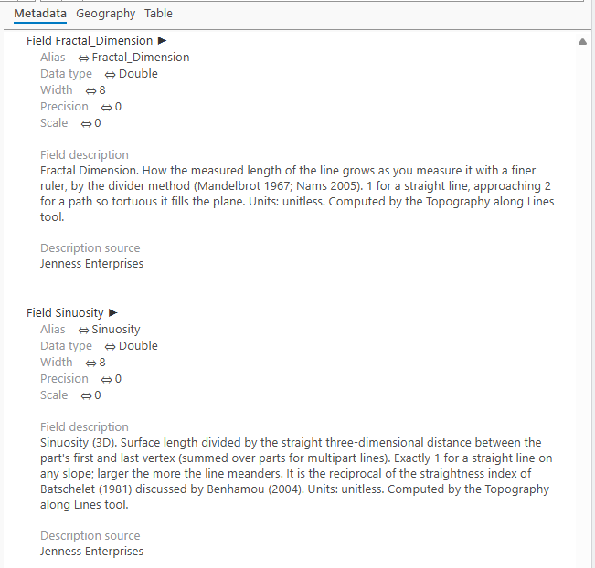
| Fractal Dimension | How the measured length of the line grows as you measure it with a finer ruler, by the divider method (Mandelbrot 1967; Nams 2005). 1 for a straight line, approaching 2 for a path so tortuous it fills the plane. | Unitless |
The fractal dimension deserves a word more, because it is the one statistic that needs a range of scales to exist. Mandelbrot's (1967) observation was that the length of the coast of Britain depends on the length of the ruler: a shorter ruler follows more of the inlets and gives a longer answer, and for a coastline this never stops. The divider method walks a pair of dividers of opening δ along the line and records the length L(δ) that results, repeats this for a series of openings, and fits a line to log L against log δ. The tool steps a fixed distance δ along the map-view path (so D keeps its classic range of 1 to 2) and measures the straight line across each step, a close variant of the classic divider walk. The smallest opening is the sampling interval, or one 512th of the line's length for a line longer than 512 intervals (about 15 km on a 30 m DEM); with the lines' own Z values it is the median spacing of their vertices. The largest is a quarter of the line's length. For a multipart line it estimates D for each part separately and reports the mean of those values, weighted by each part's surface length:
In the notation of calculus the same equation is written
where “d” stands for “a small change in”, so the fraction is a rate of change: the slope of log L against log δ. It does not mean that D is worked out at a single opening; the tool estimates that slope from the line fitted across all of them.
For a straight line the measured length does not change with the opening, the slope is 0 and D = 1. For a line whose length doubles every time the opening is cut to a quarter, the slope is −0.5 and D = 1.5. Because the fit needs at least four opening sizes between the sampling interval and a quarter of the line, a line has to be longer than roughly six times the sampling interval (about 180 m on a 30 m DEM) for D to be estimated at all; shorter lines are left null in the field, and the tool reports how many were skipped. A shapefile field cannot hold a null, so when the input is a shapefile every undefined value is written as −999 instead: Fractal Dimension on a short line, the circular standard deviation when the headings cancel exactly, and every requested statistic of a line with no usable segment. Filter those values out before analyzing a shapefile's fields, or keep the input in a geodatabase, where a true null is stored. Benhamou (2004) goes further, arguing that animal search paths are not truly fractal and that an apparent fractal dimension changes with the scale of measurement. Treat the value as meaningful only over the range of scales the sampling covers. Note that the Sinuosity statistic here is the reciprocal of the straightness index, which Benhamou finds reliable for goal-directed paths; it is not his own sinuosity index. For the example line D = 1 exactly; its sinuosity is 1 as well, and its total curvature is 0.
Units
Lengths are reported in the Length Unit you choose (meters, kilometers, feet, miles, yards or nautical miles). Elevation statistics are reported in the elevation units of the DEM or of the Z values, meters or feet, never converted to the length unit, so a line measured in miles over a DEM in meters gets its gain in meters. Slopes follow the rule above. Directions and their standard deviations are in degrees. Ratios, proportions, sinuosity, variances, the mean resultant length, the Rayleigh p-value and the fractal dimension are unitless, and the reversal count is an integer. The metadata of every field the tool creates states its units and, for the direction-dependent statistics, the direction-of-travel convention, so a field found in the table a year from now still explains itself.
The elevation units are read from the DEM's vertical coordinate system, or from the feature class's when using its own Z values, and locked; you are asked to choose meters or feet only when the data do not say. A DEM or a Z-enabled feature class in geographic coordinates (latitude and longitude) is always taken to be in meters, whatever its vertical coordinate system says. Getting this right matters: a DEM in feet treated as meters makes every elevation change 3.28 times too large.
Lengths are measured at sea level. Geodesic distances are computed on the surface of the spheroid, and a line that keeps the same latitude and longitude but lies 7,000 feet up is on a slightly bigger sphere, so it is slightly longer than the same line at sea level. The tool ignores this, as every GIS does when it measures a geodesic distance, and here is why it is safe to. The stretch is the elevation divided by the Earth's radius. At the Grand Canyon's latitude the spheroid's radius of curvature is about 6,371.5 km, so a 1 km segment raised 7,000 feet (2,134 m) becomes 1,000.335 m, 33.5 cm longer, or 0.033%. That is less than the surface-length effect of a 1.5° slope on the same segment, and far inside the accuracy of any DEM. So the planimetric length is the sea-level geodesic distance between the segment's ends, the surface length is the hypotenuse of that and the elevation change, and the elevation itself enters only through the vertical leg.
A tour of the dialog
The example runs the tool on the Crystal to South Bass trail from the profile above, with the same Grand Canyon DEM as the other pages in this group.
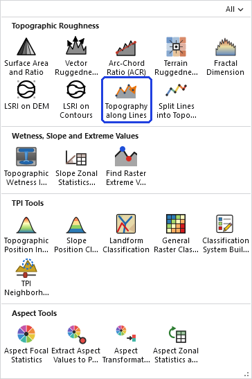
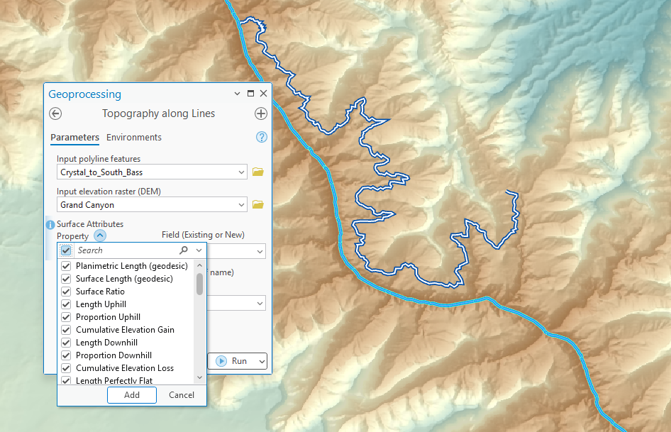
The dialog begins with the polyline feature class. If a selection is active, only the selected features are processed, the standard behavior for a feature layer input. The Elevation source offers the polylines' own Z values only when the feature class is Z-enabled; otherwise it is set to DEM raster for you and the DEM parameter becomes required. Elevation units follow.
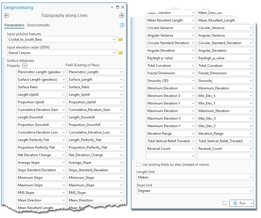
The heart of the dialog is the Surface Attributes grid, which works like Calculate Geometry Attributes. Each row pairs a Property, one of the 36 statistics, with the Field it will be written to. The Property column comes first on purpose: its down-arrow opens a checklist in which you can tick as many statistics as you like at once, and a row appears for each. Every new row's field name is filled in automatically from the property (Surface Length becomes Surface_Length, Rayleigh p-value becomes Rayleigh_p_value, and the four coordinate statistics get compact ten-character names such as Min_Elev_X), and you may edit any of them. When the input is a shapefile, whose field names are limited to ten characters, the tool fills in a short name instead: Surface Length becomes SurfLen, Cumulative Elevation Gain becomes ElevGain, Mean Resultant Length becomes MeanResLen, and so on, all of them distinct within the limit. If you change the input from a shapefile to a geodatabase feature class or back, the names the tool filled in are swapped to the other set, while any name you typed yourself is left alone. The Field column's dropdown also lists the input's existing editable numeric fields, in the order they appear in the table, so you may direct a statistic into a field you already have, or type a new name; new fields are created as double-precision numbers, or as a long integer for the reversal count. Turn on List existing fields by alias to pick existing fields by their aliases instead of their names; in that mode, a new value you type becomes a properly named field with your text as its alias.
The dialog checks your choices before you run. Pointing a statistic that can be fractional at an existing integer field is flagged, because the value would be rounded. Two rows that resolve to the same field block the run until you fix them, and this check understands shapefiles: a shapefile truncates field names to ten characters, so Cumulative_Elevation_Gain and Cumulative_Elevation_Loss would both become Cumulative and collide. The tool warns you when a name you typed will be truncated and refuses to run when two truncated names coincide, rather than silently overwriting one statistic with another. A geodatabase feature class has none of these limits, and is the better home for the output whenever you have the choice.
The remaining parameters are the Length Unit and the Slope Unit, the latter enabled only when Average, Minimum or Maximum Slope is chosen; the standard deviation and RMS of slope are always in degrees.
ModelBuilder
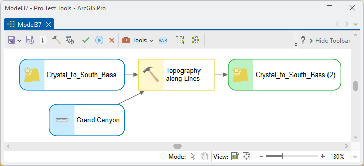
Because the tool writes fields into its input rather than creating a new dataset, it echoes the input polylines as a derived output once the fields exist. Connect that output to the next tool in your model so the downstream step runs only after the attributes have been written.
Parameters
| Label | Explanation | Data type |
|---|---|---|
| Input polyline featuresRequired · in_lines | The polyline feature class to add topography attributes to; the fields are written into this dataset. If a selection is active, only the selected features are processed. | Feature Layer |
| Elevation sourceRequired · elev_source | Z values from the polylines uses the lines' own vertex Z values (Z-enabled feature classes only; each vertex becomes a segment end). DEM raster samples elevation from a DEM. Set to DEM automatically when the input is not Z-enabled. | String |
| Input elevation raster (DEM)Optional · in_dem | The DEM to sample when the elevation source is DEM. Sample points are placed at the smaller of the cell width and height, projected into the DEM's coordinate system, and interpolated bilinearly; the DEM itself is never projected. | Raster Layer |
| Elevation unitsOptional · elev_units | Meters or Feet, for the DEM or the Z values. Filled in and locked from the vertical coordinate system when it defines them, and locked to Meters for data in geographic coordinates; asked only otherwise. | String |
| Surface AttributesRequired · surface_attributes | Rows pairing a Property (statistic) with the output Field. Use the Property column's checklist to add several at once; field names auto-fill and can be edited; the Field dropdown also lists the input's existing editable numeric fields. | Value Table |
| List existing fields by alias (instead of name)Optional · use_aliases | When on, the Field dropdown shows aliases; selecting one writes to that field, and typing a new value creates a properly named field with your text as its alias. | Boolean |
| Length UnitRequired · length_unit | Meters, Kilometers, Feet, Miles, Yards or Nautical Miles, for every length statistic. Elevation statistics stay in the elevation units. | String |
| Slope UnitOptional · slope_unit | Degrees or Percent, for Average, Minimum and Maximum Slope. The standard deviation and RMS of slope are always in degrees. Enabled only when Average, Minimum or Maximum Slope is selected. | String |
| Updated input features (derived)Derived · out_lines | The input polylines, echoed after the fields are written, for sequencing in ModelBuilder. | Feature Layer |
Python
import arcpy
arcpy.ImportToolbox(r"C:\path\to\JennessEnterprisesTools.pyt")  # your install path
# Five attributes from a DEM. Each row of surface_attributes is
# [property, field], property first; the property strings must match
# the dialog's labels exactly.
arcpy.jenness.TopographyAlongLines(
    in_lines=r"C:\Project\Trails.gdb\trails",
    elev_source="DEM raster",
    in_dem=r"C:\Project\Elev.gdb\DEM",
    elev_units="Meters",
    surface_attributes=[
        ["Surface Length (geodesic)", "SurfLen"],
        ["Surface Ratio", "SurfRatio"],
        ["Cumulative Elevation Gain", "ElevGain"],
        ["Average Slope", "AvgSlope"],
        ["Sinuosity (3D)", "Sinuosity"]],
    use_aliases=False,
    length_unit="Meters",
    slope_unit="Degrees")
The valid property strings are the 36 statistic names as they appear in the tables above, spelled exactly as in the dialog: "Planimetric Length (geodesic)", "Surface Length (geodesic)", "Surface Ratio", "Length Uphill", "Proportion Uphill", "Cumulative Elevation Gain", "Length Downhill", "Proportion Downhill", "Cumulative Elevation Loss", "Length Perfectly Flat", "Proportion Perfectly Flat", "Net Elevation Change", "Average Slope", "Slope Standard Deviation", "Minimum Slope", "Maximum Slope", "RMS Slope", "Mean Direction", "Mean Resultant Length", "Circular Variance", "Angular Variance", "Circular Standard Deviation", "Angular Deviation", "Rayleigh p-value", "Total Curvature", "Fractal Dimension", "Sinuosity (3D)", "Minimum Elevation", "Minimum Elevation X", "Minimum Elevation Y", "Maximum Elevation", "Maximum Elevation X", "Maximum Elevation Y", "Elevation Range", "Total Vertical Relief Traveled" and "Reversal Count". The elevation source is "DEM raster" or "Z values from the polylines"; the slope unit is "Degrees" or "Percent".
Recommended citation
Credits and references
By Jeff Jenness, Jenness Enterprises (www.jennessent.com). The directional statistics use the formulas from my article Issues with Directional Data (Jenness 2012), which follow Mardia and Jupp, Fisher and Batschelet; the surface-length idea is the one-dimensional version of the surface area method in Jenness (2004).
- Batschelet, E. 1981. Circular Statistics in Biology. Academic Press, London. ISBN 0-12-081050-6.
- Benhamou, S. 2004. How to reliably estimate the tortuosity of an animal's path: straightness, sinuosity, or fractal dimension? Journal of Theoretical Biology 229:209–220. doi.org/10.1016/j.jtbi.2004.03.016
- Esri. Flip Line (Editing) tool reference, ArcGIS Pro. pro.arcgis.com/.../editing/flip-line.htm. Accessed on 28 September 2026.
- Fisher, N. I. 1993. Statistical Analysis of Circular Data. Cambridge University Press, Cambridge. doi.org/10.1017/CBO9780511564345
- Greenwood, J. A., and D. Durand. 1955. The distribution of length and components of the sum of n random unit vectors. Annals of Mathematical Statistics 26:233–246. doi.org/10.1214/aoms/1177728540
- Jenness, J. S. 2004. Calculating landscape surface area from digital elevation models. Wildlife Society Bulletin 32:829–839. jennessent.com/downloads/WSB_32_3_Jenness.pdf
- Jenness, J. 2012. Issues with directional data. Remotely Wild, newsletter of the Spatial Ecology and Telemetry Working Group of The Wildlife Society. PDF
- Mandelbrot, B. B. 1967. How long is the coast of Britain? Statistical self-similarity and fractional dimension. Science 156:636–638. doi.org/10.1126/science.156.3775.636
- Mardia, K. V., and P. E. Jupp. 2000. Directional Statistics. Wiley, Chichester. doi.org/10.1002/9780470316979
- Nams, V. O. 2005. Using animal movement paths to measure response to spatial scale. Oecologia 143:179–188. doi.org/10.1007/s00442-004-1804-z
- Zar, J. H. 1999. Biostatistical Analysis, 4th edition. Prentice Hall, Upper Saddle River, New Jersey.
Licensing information
Works at every ArcGIS Pro license level (Basic, Standard, Advanced). No extension licenses are required; elevation sampling and all statistics are computed internally, without Spatial Analyst or 3D Analyst.
Related tools and pages
- About Topographic Roughness — choosing among the nine roughness measures, and why a route and a landscape are different questions.
- Split Lines into Topography Segments — the companion tool: the same segments written out as their own three-dimensional features, for symbolizing or summarizing yourself.
- Surface Area and Ratio — the surface ratio for cells instead of lines.
- Fractal Dimension — the fractal dimension of a surface (2 to 3) rather than of a path (1 to 2).
- About Aspect — the circular statistics behind the Direction group, explained at length.
- Aspect Zonal Statistics as Table — the same circular statistics for the cells of an aspect raster, zone by zone.
- Projecting Rasters — why this tool projects the sample points into the DEM rather than the DEM to the points.