

Split Lines into Topography Segments
Summary
Converts each polyline into a new PolylineZ feature class with one true three-dimensional feature per straight segment, carrying whichever per-segment attributes you choose (coordinates, lengths, slope, bearing, the turning angles between consecutive segments, and more) plus any fields copied from the source table. This is the companion to Topography along Lines: where that tool summarizes each whole line into fields on the line, this one hands you the pieces the summary was built from, so you can symbolize the segments by slope or direction, display them in space in a Scene, or compute your own statistics on any subset. No Spatial Analyst or 3D Analyst license is needed.
Why split the lines
Topography along Lines answers questions about a line as a whole: its total climb, its average slope, its mean heading. Just as often the question is about parts of a line. Which stretches of the trail are steeper than 20°? How much of the elk's track was uphill and heading north? What does the route look like when the climbs are drawn in red and the descents in blue, floating at their true elevation over the terrain in a Scene? For those you need the segments themselves, each with its own attributes, and that is what this tool writes. Every straight piece of every line becomes a two-vertex feature with real Z values at both ends, so it draws in three dimensions, and with as many of the 31 per-segment attributes attached as you like. Because every segment also carries the ObjectID of the line it came from, you can always group the pieces back into their lines with a Summary Statistics tool and compute exactly the statistic you want, on exactly the subset you want, in whatever way Topography along Lines does not already offer.
How the segments are made
The segmentation follows the same rules as Topography along Lines, so with the default segmentation and the same DEM the two tools cut a line at the same places; the At the vertices only mode described below has no counterpart there. If the input is Z-enabled you may use its own vertex elevations, in which case each existing vertex is a segment end. Otherwise a DEM is sampled: sample points are placed along each line at a ground interval equal to the smaller of the DEM's cell width and cell height, every original vertex is kept so that real bends fall on segment ends rather than being rounded across, and each point is projected into the DEM's coordinate system and its elevation interpolated bilinearly from the four surrounding cell centers. The DEM itself is never projected (see Projecting Rasters). Each vertex-to-vertex leg is cut into the fewest equal pieces that are no longer than the interval: on a 30 m DEM a straight 300 m line becomes ten 30 m segments, a 45 m leg to a corner two segments of 22.5 m, and a 61 m leg three of 20.3 m.
The output features are written in the source polylines' coordinate system, with Z taken from the sampled elevation, so Begin X and Begin Y really are coordinates in your dataset even when the DEM lives in another projection. The feature class is created as a true PolylineZ, and when the DEM has a known vertical coordinate system it is given that vertical coordinate system too (when the DEM's is unknown but the input lines have a known one, theirs is used, as it is when the lines supply their own Z values), which lets a Scene place the segments at their correct heights instead of warning that the layer has no vertical coordinate system. An unknown vertical coordinate system is not carried over, for a reason explained under Datums, transformations and a shift to watch for. Multipart lines are handled part by part, and no segment ever bridges the gap between disconnected pieces.
A sample point that falls on NoData or outside the DEM breaks the chain: the segments touching it are not written, and the segment after the gap is treated as the first of a new run for the angle fields described below. The Topography along Lines tool breaks its chain at the same gaps, so its per-line statistics never span one either. The run messages report how many segments were skipped on NoData and at how many gaps the chain was broken.
Direction of travel
Every segment is described in the direction of its line's geometry, from the line's first vertex toward its last. The signed fields (Relative Elevation Change, Relative Slope, Deflection Angle and Inclination Angle) are positive or negative according to that direction, and the Slope Direction Class calls a segment Uphill or Downhill on the same basis. A line digitized from the summit down will show every segment as downhill. If that is not the direction you mean, reverse the lines first.
The segment attributes
The Property list offers 31 attributes, grouped below. Each row you add creates one field, named with a Seg_ prefix by default (Seg_Surface_Length, Seg_Bearing, Seg_3D_Deflection_Angle and so on) so that a segment field can never be confused with a field created by Topography along Lines or with a field copied from the source table. You may rename any of them.
| Attribute | Definition | Units |
|---|---|---|
| Begin X, Begin Y, Begin Z; End X, End Y, End Z; Midpoint X, Midpoint Y, Midpoint Z | The coordinates of the segment's start, end and midpoint. X and Y are in the dataset's coordinate system; Begin Z and End Z are the sampled elevations. The midpoint's X, Y and Z are the plain means of the two ends, so Midpoint Z equals Mean Elevation, and on latitude-longitude data Midpoint X and Y are means of degrees. | Coordinate units; elevation units for Z |
| Mean Elevation | The mean of the segment's two end elevations. | Elevation units |
| Planimetric Length (geodesic) | The horizontal length of the segment, measured on the spheroid. | Length unit |
| Surface Length (geodesic) | The true three-dimensional length: the hypotenuse of the planimetric length and the elevation change. | Length unit |
| Surface Ratio | Surface length divided by planimetric length; 1 on a level segment. | Unitless |
| Relative Elevation Change | End elevation minus start elevation: positive uphill, negative downhill. | Elevation units |
| Net Elevation Change | The absolute value of the relative change. | Elevation units |
| Relative Slope | The segment's slope with its sign: positive climbing, negative descending. | Slope unit |
| Absolute Slope | The segment's steepness regardless of direction. | Slope unit |
| Average Landscape Slope | The slope of the terrain itself under the segment, as distinct from the slope of the segment: the DEM's slope from the 3 × 3 cells around points along the segment (both ends, and points at the DEM's cell interval between them), averaged. A segment running along a contour has a slope of zero but a landscape slope as steep as the hillside it crosses. Needs a DEM, even when the elevations come from the polylines' own Z values. | Slope unit |
| Average Landscape Compass Direction | The aspect of the terrain under the segment: the downslope compass direction of the DEM's surface, sampled at the same points and averaged as directions, that is, as a vector mean, so that 350° and 10° average to north rather than to 180°. Empty where the ground is flat. Needs a DEM. | Degrees |
| Traverse Angle | The angle between the segment's direction of travel and the fall line of the terrain under it, 0 to 90°: 0 when the segment runs straight up or down the slope, 90 when it follows the contour. Computed from the Bearing and the Average Landscape Compass Direction. Empty where the ground is flat. Needs a DEM. | Degrees |
| Bearing | The segment's compass azimuth, 0 to 360° clockwise from north, in the direction of travel. | Degrees |
| Deflection Angle, Absolute Deflection Angle | The horizontal turn from the previous segment: this segment's bearing minus the previous one's, wrapped to the range −180° to +180° so that a right turn is positive and a left turn negative. The absolute version drops the sign. | Degrees |
| Inclination Angle, Absolute Inclination Angle | The vertical turn from the previous segment: this segment's pitch (its signed slope angle) minus the previous one's. Positive where the route steepens upward or eases off a descent; negative where it eases off a climb or steepens downward. | Degrees |
| 3D Deflection Angle | The full three-dimensional angle between the previous segment's vector and this one's, from the dot product of the two: 0° when the route continues straight at the same pitch, 180° for an exact reversal. Always positive. | Degrees |
| Source Line ID | The ObjectID of the polyline this segment came from, for grouping segments back to their lines and for joins. | Integer |
| Segment Number, Part Index | The segment's order within its part, counted from 1 and restarting at 1 in each part of a multipart line, so the first piece of every part is always Segment Number 1; a NoData gap inside a part does not restart the count. Part Index is which part of a multipart line the segment belongs to, counted from 0. | Integer |
| Slope Direction Class | Uphill, Downhill or Flat (exactly zero elevation change), ready for symbolizing. | Text |
| Station (distance along line) | The cumulative planimetric distance from the start of the part to the start of this segment, the way a road or transect is stationed. The station keeps counting through a NoData gap, so after the gap it is still the true distance from the start of the part. | Length unit |
A worked example makes the three angle fields concrete. Take a line on a 30 m DEM whose first segment runs 30 m due north on level ground and whose second segment turns and runs 30 m due east while climbing 3 m. The second segment's bearing is 90° and its pitch is arctan(3/30) = 5.71°. Its Deflection Angle is 90° − 0° = +90°, a right turn; its Inclination Angle is 5.71° − 0° = +5.71°, because the route went from level to climbing; and its 3D Deflection Angle is 90.0°, the angle between a vector pointing north and one pointing east and slightly up (the climb does not change it, because the first segment is horizontal and the two are perpendicular in plan). The first segment has no predecessor, so all three of its angle fields are empty.
That emptiness is worth a sentence. The three angle fields
need a preceding segment, so the first segment of every line, of
every part, and of every run after a NoData gap has no value for
them. In a geodatabase that is stored as a true null. A shapefile
cannot store null in a numeric field, so there every undefined
value is stored as −999: the three angle fields where no
predecessor exists, the Average Landscape Compass Direction and
Traverse Angle on level ground, all three landscape attributes
where the DEM has no data, and the Surface Ratio of a zero-length
step. The tool detects the output format and does the right
thing, but if you are summarizing shapefile output, exclude the
−999 values first. The R script in the case study below
tests for missing values with is.na() and uses the
Seg_ field names, so it expects geodatabase output. A geodatabase
is the better home for this output.
The three landscape attributes describe the ground rather than the route, and they are there to be compared with the route. Bearing says which way the segment heads; Average Landscape Compass Direction says which way the hillside falls; the Traverse Angle is the difference between them, folded so that 0 means straight up or down the fall line and 90 means along the contour. Average Landscape Slope says how steep that hillside is, so you can ask whether an animal turns more nearly to the contour as the ground gets steeper; the section Analyzing a path below works that question through. The slope and aspect are the same quantities Esri's Slope and Aspect tools compute from a 3 × 3 neighborhood; on a geographic DEM the cell width is taken at each row's own latitude.
Units
Coordinates are in the dataset's coordinate system units. Lengths and station are in the Length Unit you choose (meters, kilometers, feet, miles, yards or nautical miles). Elevation change, Z and mean elevation are in the DEM's or the polylines' elevation units, meters or feet, read from the vertical coordinate system and asked for only when it does not say. Relative, absolute and landscape slope are in the Slope Unit you choose, degrees or percent, computed in degrees and converted only for reporting (percent = 100 × tan of the angle, with the angle in radians: every trigonometric function in ArcGIS Pro, in the Raster Calculator, the Spatial Analyst Tan tool, the Field Calculator and Arcade, takes radians, so multiply degrees by π/180 before applying it). Bearings, the landscape compass direction and all angles are in degrees. Every field's metadata states what the field is, its units and, for the direction-dependent fields, the direction convention.
Datums, transformations and a shift to watch for
Two things happen when the polylines and the DEM are on different datums, say NAD 1927 lines over a NAD 1983 DEM, and the tool handles one of them for you and warns you about the other.
Placing the sample points on the DEM. The sample points must be moved onto the DEM's datum before its elevations can be read, and that takes a geographic transformation; in the southwestern United States the NAD 1927 to NAD 1983 shift is on the order of 80 m west and 200 m north. The tool uses the transformation named in the Geographic Transformations environment when one applies to the pair, and otherwise Esri's recommended transformation for that pair and place, the same one the Project tool would suggest. It reports the one it used in its messages, and the dialog shows a warning as soon as it sees the two datums differ. The output geometry itself is never transformed: the segments are written in the polylines' own coordinate system, on the lines exactly.
The shift you may see anyway. Open the output in a map whose datum differs from the polylines' and the segments can draw offset from the lines they were cut from, as in the picture below, even though on disk they coincide to the millimeter. It happens when the output carries a vertical coordinate system, which it does when the DEM has a known one. A map applies a datum transformation to a layer that has only a horizontal coordinate system, but files a layer that also has a vertical one under a separate three-dimensional transformation, and when it cannot find a vertical component for that pair, the usual case, it draws the layer with no transformation at all rather than falling back to the horizontal one. Map Properties shows the problem plainly, in the second picture: the same NAD 1927 pair appears twice, once with no vertical coordinate system and a transformation chosen, once with a vertical coordinate system and none.
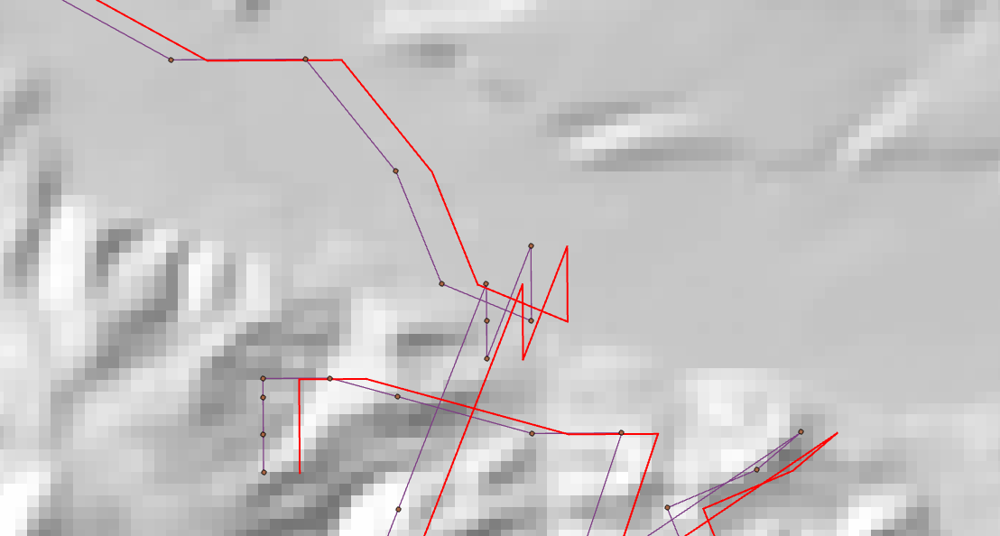
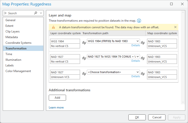
What to do about it. If the DEM's vertical coordinate system is unknown, nothing: the tool does not carry an unknown vertical coordinate system onto the output, because it conveys nothing and causes exactly this, and the output then draws where it should (if the input lines have a known vertical coordinate system of their own, the output takes that one instead). When the DEM has a real vertical datum, such as NAVD 88, the output keeps it for the sake of Scenes, and if the segments then draw shifted in a map, open Map Properties, Transformation, and choose a transformation for the pair, or set the map's own vertical coordinate system so that a three-dimensional path exists. The tool's run messages say whether a vertical coordinate system was attached and remind you of this when the datums differ.
A tour of the dialog
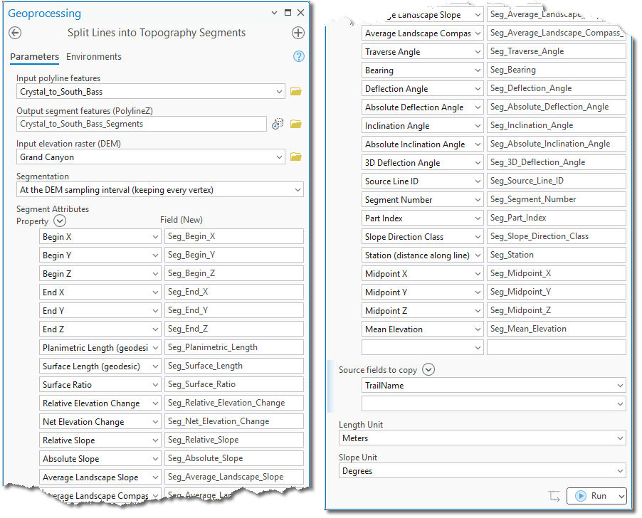
The dialog opens with the input polylines (an active selection limits the run to the selected features) and the output feature class, for which a name is suggested from the input. Save it in a geodatabase to get true nulls in the first-segment angle fields. Then the elevation source, the DEM and the elevation units, all behaving exactly as in Topography along Lines: the polylines' own Z values are offered only for a Z-enabled input, and otherwise the source is set to DEM for you. One difference: if you choose Average Landscape Slope, Average Landscape Compass Direction or Traverse Angle, the DEM is asked for even when the elevations come from the polylines' own Z values, because those three are read from the DEM's surface.
Next comes Segmentation, which applies when a DEM is sampled. The default cuts each line at the DEM's cell interval, keeping every vertex, so that a segment is never longer than a cell. At the vertices only writes exactly one segment per vertex pair, with the elevation sampled at the vertices, and is the appropriate setting for a GPS track: each step between fixes becomes one feature, with the landscape slope and aspect averaged along the whole step. The reason is that you only really know where the animal was at the fixes. The straight line between two fixes is a guess at the route it took, so sampling the DEM every cell along that line would describe terrain the animal may never have crossed, and would turn one observation into dozens of records. Lines that supply their own Z values are vertex to vertex already, so the choice is disabled for them.
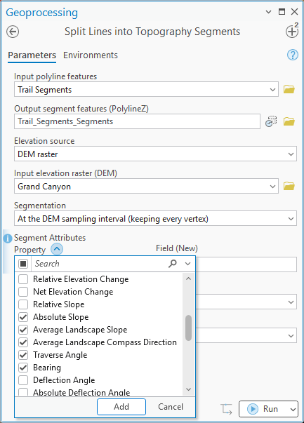
The Segment Attributes grid works like the Surface Attributes grid of the companion tool. The Property column's down-arrow opens a checklist; tick as many attributes as you like, a row appears for each, and its field name is filled in with the Seg_ prefix, or, when the output will be a shapefile, with short names within the ten-character limit (SgSurfLen, SgBearing, SgDefl3D and so on); the tool swaps between the two sets if you change the output from one kind of dataset to the other. Edit any name you wish. Fields are created with the right type for each attribute: double-precision numbers for the measurements, long integers for the Source Line ID, Segment Number and Part Index, and text for the Slope Direction Class. The grid is optional; with no rows the tool still writes the bare three-dimensional segment features.
Source fields to copy is a second checklist, this one of the input table's fields. Any field you tick is copied onto every segment of its line, so a trail name, a route class or an animal ID travels with the pieces and you can select or summarize by it directly. Copied fields keep their type and, wherever legal, their name; a name that would be invalid, reserved (such as Shape_Length) or a duplicate of another output field is adjusted automatically, and the tool tells you when it does. Then the Length Unit, and the Slope Unit when a slope attribute is chosen.
Last, a collapsed group, Advanced: alternative steps for
step-selection analysis, which comes alive when the elevation
is from a DEM and Segmentation is At the vertices only. Give
it a number of alternative steps per real step, 10 or 35 are usual,
and the tool casts that many steps from the start point of every
real step, evenly spaced around the compass from a random offset or
at random headings, each as long as the real step or as long as a
step drawn at random from the same line. Every alternative is a
real feature that goes through the same engine, so its elevations,
path angle, landscape slope, aspect, traverse angle and copied
fields are measured on the ground it actually crosses. Three fields
tie the output together: Seg_Used, 1 for a real step and 0
for an alternative; Seg_Step_ID, one number per real step
shared by its alternatives; and Seg_Alt_Number, 0 for the
real step and 1 to K for the alternatives (SgUsed, SgStepID and
SgAltNum in a shapefile). Because each alternative is built as a
standalone two-point line, its Deflection, Inclination and 3D
Deflection angles are always empty (−999 in a shapefile),
its Segment Number is 1, its Part Index 0 and its Station 0; a
turn-angle covariate for a step-selection model therefore has to
come from the real steps. A seed makes the run
reproducible. The output grows K + 1 times, and the
symbology colors the alternatives too; a definition query
Seg_Used = 1 shows the track alone. Alternatives that
end on NoData or off the DEM are dropped and counted in the
messages; so, separately, are the alternatives not cast because
their real step has zero length.
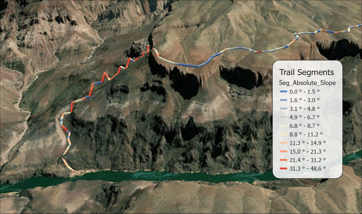
When the output reaches the map it is already symbolized: an Unclassed Colors renderer on a blue-to-yellow-to-red ramp, keyed to the most useful of the attributes you actually calculated, in this order of preference: Mean Elevation, then Begin X, End X, Absolute Slope, Relative Slope, and if none of those was chosen, the first attribute in your grid. Change the field, classification method and color ramp in the Symbology pane to see the segments symbolized in any manner you want.
Three examples of what you can do with these segments
- Symbolize the route. Color the segments by Relative Slope with a diverging ramp and the climbs and descents of a trail appear at a glance; color by Bearing to see which way each stretch heads; select the Uphill class and see at once how much of the route is climbing.
- Compute your own statistic. Topography along Lines offers 36 statistics, but not, for instance, the length of trail steeper than 20°, or the mean bearing of only the downhill segments. Select the segments that meet your condition, run Summary Statistics with Source Line ID as the case field, and join the result back to the original lines.
- Look at it in space. Add the feature class to a Scene over the same DEM and the segments draw at their sampled elevations. A route up a steep face is easier to read from the side than from above.
Analyzing a path: which way does an animal cross a hillside?
Here is one question the segments can answer, worked from the field data to the statistics. Picture an animal on a steep hillside. It is probably not walking straight down the cliff; it is more likely to angle across it, and the steeper the ground the more nearly it should follow the contour. That is a hypothesis about three numbers per step: the direction of travel, the direction the hillside faces, and how steep the hillside is.
The idea has been tested. Dunford et al. (2020) followed pumas with GPS fixes every five minutes over a DEM and defined three angles: the topographical slope angle, the steepness of the hill; the path angle, the steepness of the route actually taken; and the traverse angle, the horizontal angle between the path and the direction of steepest slope (the aspect), also known as the fall line. Their pumas crossed hills averaging 17.2° on paths averaging only 7.3°, and they modeled the traverse angle against slope with mixed models that treated each puma as a random effect. Redcliffe et al. (2025) took the same question to six ungulate species, three wild and three domestic, in three French mountain ranges, using collars that combined GPS with accelerometers and magnetometers, and found that "animals travelled obliquely so that the angle that any individual experienced was lower than that of the topography", with differences among species. Both sit inside the energy-landscape framework of Shepard et al. (2013), which argues that slope is the main driver of the cost of moving and therefore of the routes animals choose. On a planar hillside the three angles are tied together: tan(path angle) = tan(slope) × cos(traverse angle). This tool writes all three, as Relative Slope, Average Landscape Slope and Traverse Angle.
Making the table. Build each animal's track as a polyline whose vertices are its GPS fixes (Points To Line, ordered by time, one line per animal or per session). Run this tool on it with the elevation from a DEM, Segmentation set to At the vertices only, and these attributes: Relative Slope, Bearing, Average Landscape Slope, Average Landscape Compass Direction, Traverse Angle, Planimetric Length and Source Line ID, plus the animal's ID copied from the source table, and, for the step-selection model below, a number of alternative steps in the Advanced group. Every step between fixes is now one record with the three angles on it, followed by its alternatives. Export the attribute table to a CSV file, and the rest is statistics, which is better done in R than in ArcGIS Pro.
Used against available. Comparing the steps an animal took with the steps it could have taken is the older idea in this workflow. Dickson, Jenness and Beier (2005) compared each cougar movement segment, for vegetation, with 35 alternative segments cast at 10° intervals around its starting point, each as long as the mean of all the movement segments in that monitoring session; and, for slope, with 100 alternative segments as long as the original, each ending at a random point within 50 m of the original's start and end points inside the movement-segment buffer, using paired tests. The Alternate Animal Movement Routes extension for ArcView 3.x (Jenness 2005) generated such alternatives three ways: by shuffling a route's own segments, by drawing segment lengths, bearings and turning angles from the route's own distributions, and by relocating or rotating the whole route. The modern form is the step-selection function (Fortin et al. 2005; Thurfjell, Ciuti and Boyce 2014): each used step is matched with random alternative steps from the same starting point, and conditional logistic regression asks which attributes made the used step the one taken. This tool's Advanced group casts those alternatives for you, measures each on the ground it crosses, and marks the table with Seg_Used and Seg_Step_ID so the model below reads it directly.
Whether to weight by length. The sample R script linked at the end of this page runs the fidelity regression and the mixed model both ways, and which is right depends on the question. Unweighted, every step is one vote however long it is, which is correct when each step is one decision, as with GPS fixes at a fixed time interval, where a longer step only means the animal moved faster. Weighted by planimetric length, the analysis describes distance traveled instead, what share of the route follows the contour, and that is the version to use when the vertices are unevenly spaced, as on a digitized trail. Planimetric length is the better weight of the two the tool offers: surface length grows with the path angle, so it would quietly favor the steep steps. The step-selection model is never weighted; its unit is the choice.
Three cautions, all from the papers above. Aspect means nothing on flat ground and little on gentle ground, so the script drops steps whose terrain slope is under 5° before it does anything; without that, noise at low slopes can masquerade as the very pattern you are looking for. Steps shorter than about twice the GPS error carry more noise than signal in their bearing, and the DEM's cell size should be small against the step length. And the steps of one animal are not independent evidence, which is why the animal enters the mixed model as a random effect and why the step-selection model is stratified by step. Uphill and downhill travel are worth analyzing separately; Relative Slope keeps the sign.
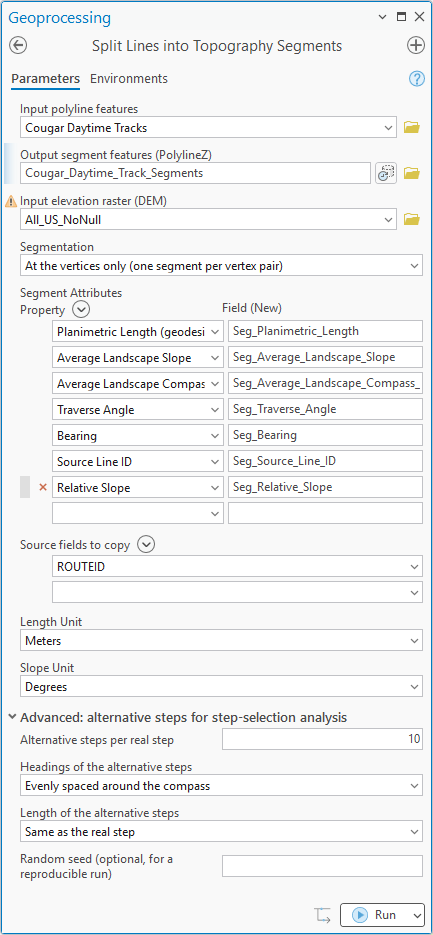
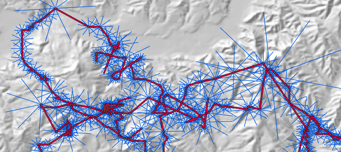
The tracks are cougar movements from the late 1980s and early 1990s: radio-telemetry locations taken every 15 minutes by a very motivated group of field techs, because following those cougars through the Santa Ana Mountains was tough work. They are the source data of Dickson, Jenness and Beier (2005). Here they are 21 daytime tracking sessions, one polyline each with a fix at every vertex, over a DEM of the range. The tool was run as in the first picture: vertices only, so each step between fixes is one segment; the seven attributes the R script needs, with Relative Slope supplying the path angle; the session number (ROUTEID) copied; and, in the Advanced group, ten alternative steps per real step, evenly spaced around the compass and as long as the real step. The second picture is the result: the real steps in red, each with its fan of ten blue alternatives, every one of them measured on the hillside it crosses.
The table was exported to a CSV file and the script run on it, with the session as the grouping variable since no animal ID was copied. The transcript, with the script's comment blocks trimmed:
> d_all <- read.csv("D:\\...\\Cougar_Segments.csv")
> names(d_all)
 [1] "Shape_Length"                            "Seg_Planimetric_Length"
 [3] "Seg_Average_Landscape_Slope"             "Seg_Average_Landscape_Compass_Direction"
 [5] "Seg_Traverse_Angle"                      "Seg_Bearing"
 [7] "Seg_Source_Line_ID"                      "Seg_Relative_Slope"
 [9] "Seg_Used"                                "Seg_Step_ID"
[11] "Seg_Alt_Number"                          "ROUTEID"
> slope_col <- "Seg_Average_Landscape_Slope"
> trav_col  <- "Seg_Traverse_Angle"
> path_col  <- "Seg_Relative_Slope"
> len_col   <- "Seg_Planimetric_Length"
> group_col <- "Seg_Source_Line_ID"
> has_alt <- "Seg_Used" %in% names(d_all)
> d <- if (has_alt) d_all[d_all$Seg_Used == 1, ] else d_all
> d$group <- factor(d[[group_col]])
> # 1. keep steps where the terrain slope is at least 5 degrees
> d <- d[!is.na(d[[trav_col]]) & d[[slope_col]] >= 5, ]
> d$path_angle <- abs(d[[path_col]])
> # 2a. fall-line fidelity index, per tracking session (unweighted)
> fidelity <- sapply(split(d, d$group), function(x)
+     coef(lm(path_angle ~ 0 + Seg_Average_Landscape_Slope, data = x)))
> print(round(fidelity, 3))
 1.Seg_Average_Landscape_Slope  2.Seg_Average_Landscape_Slope  3.Seg_Average_Landscape_Slope
                         0.544                          0.275                          0.547
 4.Seg_Average_Landscape_Slope  5.Seg_Average_Landscape_Slope  6.Seg_Average_Landscape_Slope
                         0.432                          0.443                          0.445
 7.Seg_Average_Landscape_Slope  8.Seg_Average_Landscape_Slope  9.Seg_Average_Landscape_Slope
                         0.477                          0.392                          0.646
10.Seg_Average_Landscape_Slope 11.Seg_Average_Landscape_Slope 12.Seg_Average_Landscape_Slope
                         0.378                          0.335                          0.401
13.Seg_Average_Landscape_Slope 14.Seg_Average_Landscape_Slope 15.Seg_Average_Landscape_Slope
                         0.351                          0.357                          0.322
16.Seg_Average_Landscape_Slope 17.Seg_Average_Landscape_Slope 18.Seg_Average_Landscape_Slope
                         0.480                          0.574                          0.436
19.Seg_Average_Landscape_Slope 20.Seg_Average_Landscape_Slope 21.Seg_Average_Landscape_Slope
                         0.373                          0.405                          0.401
> # 3a. traverse angle against terrain slope, session as a random effect
> m <- lmer(Seg_Traverse_Angle ~ Seg_Average_Landscape_Slope + (1 | group),
+           data = d)
boundary (singular) fit: see help('isSingular')
> print(summary(m)$coefficients)
                              Estimate Std. Error   t value
(Intercept)                 41.9016103   2.697973 15.530775
Seg_Average_Landscape_Slope  0.7200162   0.176686  4.075118
> nlevels(d$group)
[1] 21
> # 4. step-selection function: each real step against its 10 alternatives
> ssf <- d_all[!is.na(d_all[[path_col]]) & !is.na(d_all[[slope_col]]), ]
> ssf$path_angle <- abs(ssf[[path_col]])
> ssf$land_slope <- ssf[[slope_col]]
> ssf$cluster_id <- ssf[[group_col]]
> ok <- tapply(ssf$Seg_Used, ssf$Seg_Step_ID, function(u) any(u == 1) && any(u == 0))
> ssf <- ssf[ssf$Seg_Step_ID %in% names(ok)[ok], ]
> fit <- clogit(Seg_Used ~ path_angle + path_angle:land_slope + strata(Seg_Step_ID)
+               + cluster(cluster_id), data = ssf, method = "efron")
> print(summary(fit)$coefficients)
                              coef exp(coef)    se(coef)  robust se         z   Pr(>|z|)
path_angle            -0.056300077 0.9452554 0.027218902 0.02289297 -2.459274 0.01392183
path_angle:land_slope  0.001240074 1.0012408 0.001348741 0.00105983  1.170069 0.24197340
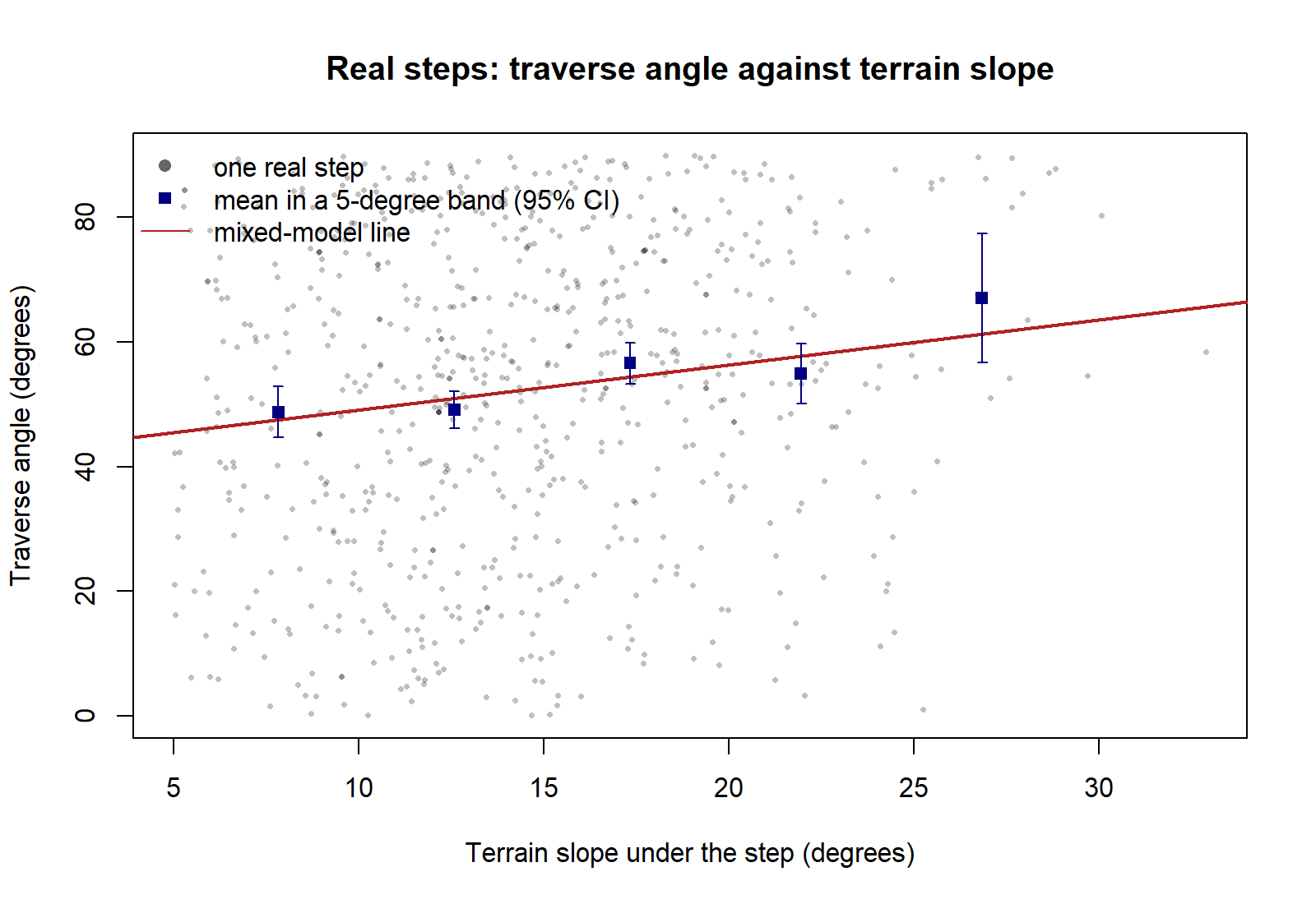
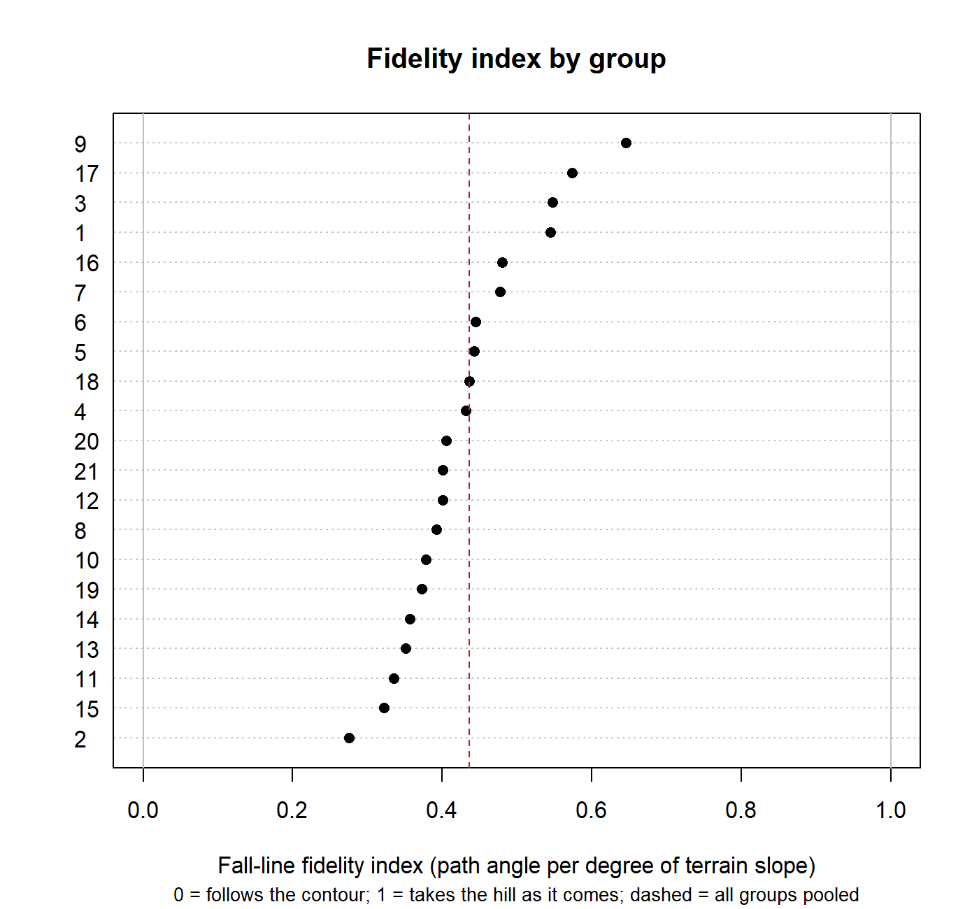
What it says. The fall-line fidelity index of the 21 sessions runs from 0.28 to 0.65: on a hillside of a given steepness, the cats' paths were between a quarter and two thirds as steep as the hillside, never as steep as the ground itself and never flat along the contour. The mixed model puts the traverse angle at about 45° on a 5° hillside, the gentlest ground in the data, rising 0.72° for every degree of terrain slope (t = 4.1), so about 63° on a 30° hillside: the steeper the ground, the more nearly the cats crossed it along the contour. The "singular fit" warning is not a defect. It reports that the session-level random effect was estimated at zero; with 21 sessions that is a finding, that once terrain slope is accounted for the sessions did not differ in their baseline traverse angle, and the fixed effects are exactly what a plain regression would give.
The script's last step draws the results, four figures in base R with nothing extra to install. The first two are the mixed model and the fidelity index:
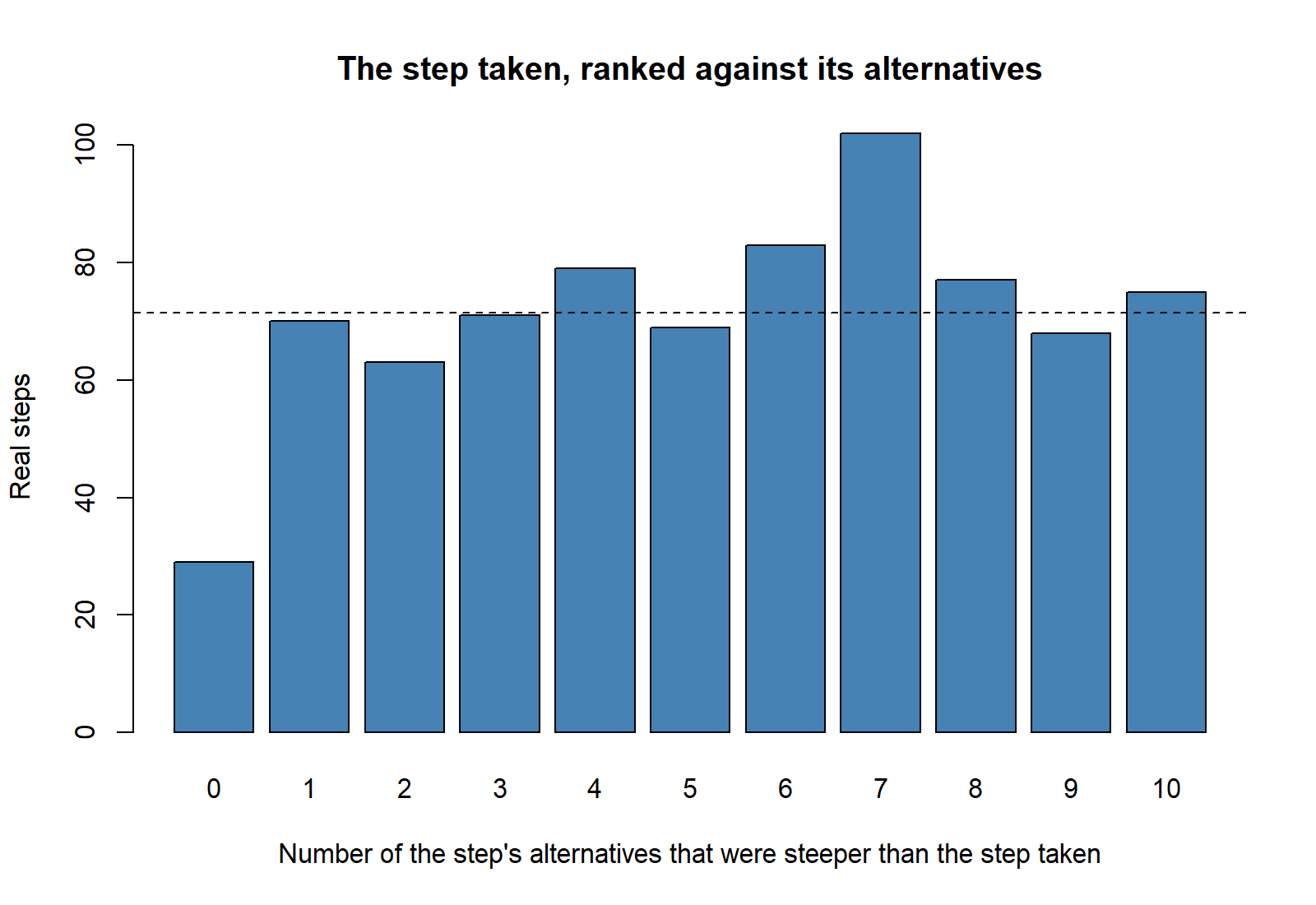
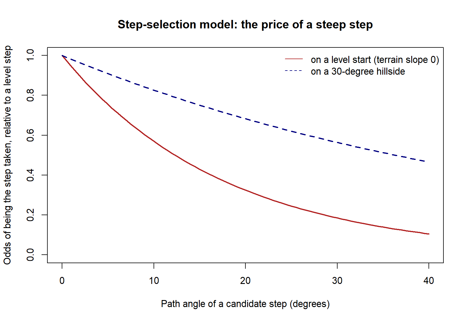
The step-selection model says the same thing from the other side. At a given start point, each extra degree of path steepness cut the odds of a step being the one taken by about 5 percent (coefficient −0.056, p = 0.014 with the cluster-robust standard error): steep options were avoided. The interaction with terrain slope is small, positive and far from significant (p = 0.24), so there is no evidence that the avoidance grew stronger on steeper hillsides; the price paid per degree of path angle looks roughly constant. The two results fit together through the geometry of the plane, path angle = arctan(tan slope × cos traverse angle): a constant dislike of steep path angles forces a larger traverse angle where the hillside is steeper, which is what the mixed model found.
The other two figures show the step-selection result, first straight from the data and then as the model's curve:
Two notes on the numbers. Consecutive steps of one session are not independent, so the model's standard errors are the cluster-robust ones, computed with the session as the cluster; here they came out a little smaller than the ordinary ones rather than larger, so the clustering cost nothing. And these are 15-minute fixes with steps of a few hundred meters over a DEM coarser than the terrain a cat responds to, so the path angle of a straight step between fixes is a smoothed version of what the animal walked, which pushes every effect toward zero. Finding the avoidance at all under those conditions is the notable part.
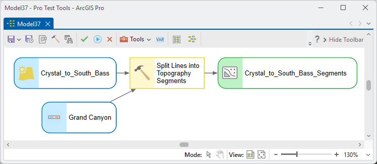
ModelBuilder
Parameters
| Label | Explanation | Data type |
|---|---|---|
| Input polyline featuresRequired · in_lines | The polyline feature class to split. If a selection is active, only the selected features are processed. | Feature Layer |
| Output segment features (PolylineZ)Required · out_fc | The new feature class: one true PolylineZ feature per straight segment, in the input's coordinate system, with the DEM's vertical coordinate system when it has a known one (otherwise the input lines' own, if known). Save to a geodatabase for true nulls; a shapefile stores −999 for every undefined value. | Feature Class |
| Elevation sourceRequired · elev_source | Z values from the polylines (Z-enabled input only) or DEM raster. Set to DEM automatically when the input is not Z-enabled. | String |
| Input elevation raster (DEM)Optional · in_dem | The DEM to sample when the elevation source is DEM; sample points are placed at the smaller of the cell width and height, projected into the DEM's coordinate system, and interpolated bilinearly. Also required, whatever the elevation source, when a landscape attribute is chosen. | Raster Layer |
| Elevation unitsOptional · elev_units | Meters or Feet, for the DEM or the Z values; locked from the vertical coordinate system when it defines them, and locked to Meters for data in geographic coordinates. | String |
| SegmentationOptional · segmentation | At the DEM sampling interval (keeping every vertex), the default, or At the vertices only (one segment per vertex pair) for lines whose vertices are GPS fixes. Applies only when a DEM is sampled. | String |
| Segment AttributesOptional · surface_attributes | Rows pairing a Property (segment attribute) with its output field. Tick several at once from the Property checklist; names auto-fill with the Seg_ prefix. With no rows, the bare segment features are still written. | Value Table |
| Source fields to copyOptional · copy_fields | Fields from the input table to copy onto every segment of each line; invalid, reserved or duplicate names are adjusted automatically. | Value Table |
| Length UnitRequired · length_unit | Meters, Kilometers, Feet, Miles, Yards or Nautical Miles, for the length and station fields. | String |
| Slope UnitOptional · slope_unit | Degrees or Percent, for Relative Slope, Absolute Slope and Average Landscape Slope. Used only when a slope attribute is selected. | String |
| Alternative steps per real stepOptional · alt_count | How many alternative steps to cast from each real step's start point, for a step-selection analysis; 0 casts none. Applies only with a DEM and vertices-only segmentation. Adds the fields Seg_Used, Seg_Step_ID and Seg_Alt_Number (SgUsed, SgStepID and SgAltNum in a shapefile). | Long |
| Headings of the alternative stepsOptional · alt_headings | Evenly spaced around the compass (from a random offset) or Random. | String |
| Length of the alternative stepsOptional · alt_length | Same as the real step or Drawn at random from the line's own step lengths. | String |
| Random seed (optional, for a reproducible run)Optional · alt_seed | Any whole number; the same seed reproduces the same alternatives. | Long |
Python
import arcpy
arcpy.ImportToolbox(r"C:\path\to\JennessEnterprisesTools.pyt")  # your install path
# Segments from a DEM with six attributes and two copied source fields.
# surface_attributes rows are [property, field], property first;
# copy_fields rows are [field].
arcpy.jenness.SplitLinesIntoSegments(
    in_lines=r"C:\Project\Trails.gdb\trails",
    out_fc=r"C:\Project\Trails.gdb\trail_segments",
    elev_source="DEM raster",
    in_dem=r"C:\Project\Elev.gdb\DEM",
    elev_units="Meters",
    segmentation="At the DEM sampling interval (keeping every vertex)",
    surface_attributes=[
        ["Mean Elevation", "Seg_Mean_Elevation"],
        ["Surface Length (geodesic)", "Seg_Surface_Length"],
        ["Absolute Slope", "Seg_Absolute_Slope"],
        ["Bearing", "Seg_Bearing"],
        ["3D Deflection Angle", "Seg_3D_Deflection_Angle"],
        ["Source Line ID", "Seg_Source_Line_ID"]],
    copy_fields=[["TrailName"], ["Trail_Class"]],
    length_unit="Meters",
    slope_unit="Degrees",
    alt_count=0)        # e.g. alt_count=35, alt_headings="Evenly spaced around the compass",
                        #      alt_length="Same as the real step", alt_seed=1 for a step-selection table
The valid property strings, spelled exactly as in the dialog, are "Begin X", "Begin Y", "Begin Z", "End X", "End Y", "End Z", "Planimetric Length (geodesic)", "Surface Length (geodesic)", "Surface Ratio", "Relative Elevation Change", "Net Elevation Change", "Relative Slope", "Absolute Slope", "Average Landscape Slope", "Average Landscape Compass Direction", "Traverse Angle", "Bearing", "Deflection Angle", "Absolute Deflection Angle", "Inclination Angle", "Absolute Inclination Angle", "3D Deflection Angle", "Source Line ID", "Segment Number", "Part Index", "Slope Direction Class", "Station (distance along line)", "Midpoint X", "Midpoint Y", "Midpoint Z" and "Mean Elevation". The elevation source is "DEM raster" or "Z values from the polylines"; the segmentation is "At the DEM sampling interval (keeping every vertex)" or "At the vertices only (one segment per vertex pair)"; the slope unit is "Degrees" or "Percent"; the alternative-step headings are "Evenly spaced around the compass" or "Random" and their length "Same as the real step" or "Drawn at random from the line's own step lengths".
Recommended citation
Credits and references
By Jeff Jenness, Jenness Enterprises (www.jennessent.com). The segment attributes are elementary geometry; the surface length follows the three-dimensional distance idea of Jenness (2004); the landscape slope and aspect use the 3 × 3 method of Esri's Slope and Aspect tools; the traverse and path angles follow Dunford et al. (2020); and the segmentation engine is shared with Topography along Lines.
- Dickson, B. G., J. S. Jenness, and P. Beier. 2005. Influence of vegetation, topography, and roads on cougar movement in southern California. Journal of Wildlife Management 69:264–276. doi:10.2193/0022-541X(2005)069<0264:IOVTAR>2.0.CO;2
- Dunford, C. E., N. J. Marks, C. C. Wilmers, C. M. Bryce, B. Nickel, L. L. Wolfe, D. M. Scantlebury, and T. M. Williams. 2020. Surviving in steep terrain: a lab-to-field assessment of locomotor costs for wild mountain lions (Puma concolor). Movement Ecology 8:34. doi:10.1186/s40462-020-00215-9
- Esri. How Slope works and How Aspect works. ArcGIS Pro tool reference. pro.arcgis.com/.../how-slope-works.htm and pro.arcgis.com/.../how-aspect-works.htm. Accessed on 28 September 2026.
- Fortin, D., H. L. Beyer, M. S. Boyce, D. W. Smith, T. Duchesne, and J. S. Mao. 2005. Wolves influence elk movements: behavior shapes a trophic cascade in Yellowstone National Park. Ecology 86:1320–1330. doi:10.1890/04-0953
- Jenness, J. S. 2004. Calculating landscape surface area from digital elevation models. Wildlife Society Bulletin 32:829–839. jennessent.com/downloads/WSB_32_3_Jenness.pdf
- Jenness, J. 2005. Alternate Animal Movement Routes, v. 2.1, an ArcView 3.x extension. Jenness Enterprises. jennessent.com/arcview/alternate_routes.htm
- Redcliffe, J., R. Wilson, M. Holton, P. Hopkins, M. Garel, P. Marchand, G. Wilson, R. Brown, and L. Börger. 2025. Steep slopes, shallow angles: mountain ungulates create their own topography through movements. Canadian Journal of Zoology 103:1–18. doi.org/10.1139/cjz-2024-0095
- Shepard, E. L. C., R. P. Wilson, W. G. Rees, E. Grundy, S. A. Lambertucci, and S. B. Vosper. 2013. Energy landscapes shape animal movement ecology. American Naturalist 182:298–312. doi:10.1086/671257
- Thurfjell, H., S. Ciuti, and M. S. Boyce. 2014. Applications of step-selection functions in ecology and conservation. Movement Ecology 2:4. doi:10.1186/2051-3933-2-4
Licensing information
Works at every ArcGIS Pro license level (Basic, Standard, Advanced). No extension licenses are required; elevation sampling, segmentation and the three-dimensional output are all handled internally, without Spatial Analyst or 3D Analyst.
Related tools and pages
- Topography along Lines — the companion tool: the same segments summarized into 36 statistics per line, with the theory behind the slope and direction measures.
- About Topographic Roughness — choosing among the nine roughness measures.
- Surface Area and Ratio — the surface ratio for cells instead of segments.
- Projecting Rasters — why the sample points go to the DEM rather than the DEM to the points.
- traverse_angle_example.R — sample R code for the analysis above: the fall-line fidelity index, the mixed model of traverse angle against terrain slope, and the step-selection model on this tool's alternative steps, and then draws the four figures of the case study. It runs on its own on simulated data; point it at your exported table instead.