

Terrain Ruggedness Index (TRI)
Summary
Computes a Terrain Ruggedness Index: for every cell of a DEM, a measure of how much the elevations in a circular neighborhood around it depart from flat. Four related measures are offered in one tool, because ruggedness means different things to different people: the root of the summed squared differences from the focal cell (the original index of Riley, DeGloria and Elliot 1999), the mean absolute difference from the focal cell (Wilson et al. 2007), a distance-weighted variant of my own that turns each difference into the slope toward that neighbor, and the standard deviation of all the elevations in the neighborhood. Higher values are more rugged in every case. All four respond to overall slope, so a smooth but steep hillside scores as rugged; if you want a measure that ignores slope, see the Vector Ruggedness Measure. The tool is correct on geographic (latitude/longitude) DEMs and needs no Spatial Analyst license.
The idea
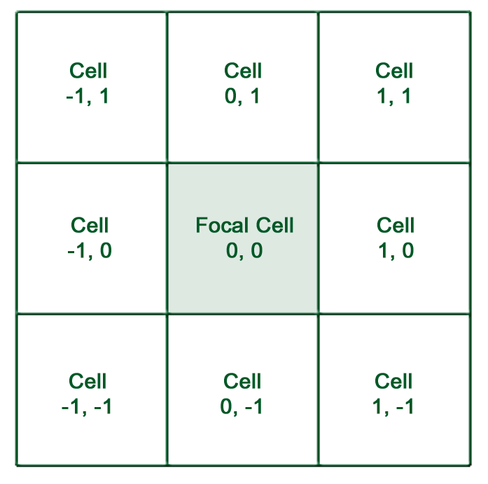
Riley, DeGloria and Elliot (1999) wanted a quick, objective number for terrain heterogeneity that could be computed over an entire state from freely available DEMs, to test whether terrain mattered to mountain lions in Montana. Their reasoning was direct: rugged terrain is terrain where the elevation changes a lot from one cell to the next. So for each cell they took the elevation difference between the focal cell and each of its eight neighbors, squared each difference, added the eight squares, and took the square root of the sum. A perfectly level neighborhood scores 0. A cell perched above all of its neighbors, or sunk below all of them, scores high. Riley et al. provide the correct formula for their version of TRI in their Figure 1, the square root of the summed squared differences, which is what this tool computes. They make a math error in the worked examples of their Figure 3, though. The values they show there (a peak and a pit both 700, a gentle surface 100) are the simple sums of the absolute differences. Under their own formula the three examples would be 250, 250 and 41.8, so the figure overstates TRI by a factor of 2.4 to 2.8. This could have serious implications for the thresholds in their final classification scheme (see below), but the general concepts they present are good. Sappington et al. (2007) computed TRI as that absolute sum. Either way a peak and its mirror-image pit score the same. As I say in the lecture, the index is reasonably intuitive, not difficult to calculate, and it does distinguish flat from sloping areas.
There are a lot of ways you can look at this question, which is why I offer four measures instead of one. The Riley formula is a sum, so it grows with the number of neighbors; a mean behaves better as the neighborhood changes. It counts a difference to a diagonal neighbor, which sits 41% farther away, exactly like a difference to an edge neighbor, even though the diagonal difference represents a gentler gradient. And it measures everything relative to the focal cell, when you might instead care about the spread of elevations in the neighborhood as a whole. Each of those observations leads to a different, defensible index, and the right one depends on the question you are asking. What all four share is a circular moving neighborhood, a radius you choose, and sensitivity to slope: a smooth steep hillside really does have elevations that differ across it, and all four say so.
The four methods, with a worked example
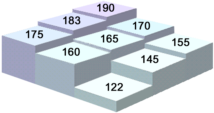
In the formulas below, z0 is the elevation of the focal cell, zi is the elevation of neighbor i, n is the number of neighbors in the neighborhood, and di is the horizontal ground distance from the focal cell center to neighbor i. For the example cell, reading down the columns from the northwest corner, the eight neighbors are 190, 170, 155, 183, 145, 175, 160 and 122, and the eight differences from the focal 165 are +25, +5, −10, +18, −20, +10, −5 and −43.
Riley et al. 1999: root of summed squared differences
Square each difference: 625, 25, 100, 324, 400, 100, 25 and 1,849. Their sum is 3,448, and its square root is 58.7 m. Notice how the one large difference, the 43 m drop to the southeast corner, contributes more than half of the total on its own; squaring makes this index very sensitive to a single extreme neighbor. The output is in the DEM's own elevation units, meters here. Riley et al. published a set of named ruggedness classes for this index: level (0 to 80 m), nearly level (81 to 116), slightly rugged (117 to 161), intermediately rugged (162 to 239), moderately rugged (240 to 497), highly rugged (498 to 958) and extremely rugged (959 to 4,367). If you are tempted to apply those numbers to your own data, keep in mind where they came from: they were an equal-area classification of Montana computed on 1 km cells in meters, and the index scales with the cell size (a 1 km cell spans far more relief than a 30 m one), so treat them as an example of how to classify rather than as thresholds to apply to your own DEM. Our example cell would be classed as level by that scheme, which tells you more about the 1 km cells it was built on than about our 100 m cell. Riley et al. also do not say whether their class limits were computed with the formula or with the absolute sums of their Figure 3, which is one more reason not to apply them to this tool's output.
Wilson et al. 2007: mean absolute difference
Take the absolute value of each difference (25, 5, 10, 18, 20, 10, 5 and 43), add them to get 136, and divide by the eight neighbors: 17.0 m. Wilson et al. (2007, p. 11) give this formula for a 3 × 3 window and used it to describe seabed terrain from multibeam bathymetry for benthic habitat mapping. They credit the adaptation of Riley's index to Valentine et al. (2004), whose ArcInfo macro they ran. They also write out a multiscale version (p. 12), the sum of the absolute differences over an n × n window divided by n2 − 1, which is the same mean this tool computes over its circular neighborhood. Because it is an average rather than a sum, it is not biased downward when a neighbor is missing at the raster edge or beside a NoData hole, and it does not balloon as the neighborhood grows the way a sum does, so it is the better choice when you intend to compare radii or work near edges. Because it does not square, the 43 m drop counts for less than it did under Riley. The output is again in the DEM's elevation units.
Slope (distance-weighted, Jenness)
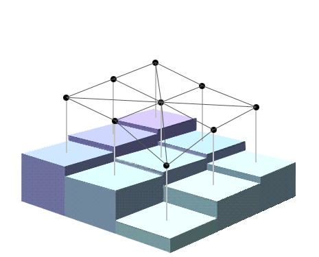
This is a variation I proposed in the lecture. The Riley and Wilson indices treat every neighbor the same, but on a 100 m grid the four diagonal neighbors are 141.4 m away while the four edge neighbors are 100 m away, so a 20 m difference to a corner is a gentler gradient than a 20 m difference to an edge. Dividing each difference by the distance to that neighbor corrects this, and doing so is mathematically the same as measuring the slope from the focal cell to each neighbor as rise over run. For the example, the four edge slopes are 5/100 = 0.050, 18/100 = 0.180, −20/100 = −0.200 and −5/100 = −0.050, and the four diagonal slopes are 25/141.4 = 0.177, −10/141.4 = −0.071, 10/141.4 = 0.071 and −43/141.4 = −0.304. Squared and summed they come to 0.2111, whose square root is 0.459. That number is a dimensionless rise over run, a measure of slope dispersion, and it is not comparable to the meter values of the other methods. To keep it dimensionless whatever the DEM's units, the tool scales elevations to meters internally for this method only, so a DEM in feet gives the same slope value as the same terrain in meters. On a geographic DEM the neighbor distances are computed per row on the spheroid, so the diagonals stay the right length at any latitude.
Keep in mind what this method was designed for. The idea was to fix one specific problem, the diagonals of the 3 × 3 window, where the far and near neighbors differ in distance by only 41% and dividing by distance simply puts all eight on an equal footing. The tool lets you use it with a larger radius, and it will do what it says, but think about what that means. The slope from the focal cell to a cell ten cells away is the average gradient across all the ground between them, with every ridge and gully along the way averaged out, so it will naturally be gentler than the slope to the cell next door. Go out far enough and everything merges with the horizon. The Grand Canyon DEM shows this clearly. The average rise over run from a cell to another cell a given distance away falls steadily as that distance grows:
| Distance to the other cell | 1 cell (28 m) | 5 cells (140 m) | 10 cells (280 m) | 20 cells (560 m) | 100 cells (2.8 km) |
|---|---|---|---|---|---|
| Mean rise over run | 0.37 | 0.32 | 0.28 | 0.23 | 0.10 |
| As an angle | 20.5° | 17.8° | 15.7° | 12.8° | 5.8° |
So in a large neighborhood the distant cells each contribute less than the near ones, which is sensible, but there are far more of them, and like the Riley index this is a sum, so the total still climbs as the radius grows. At the default 1.5 cells the method does exactly the job it was invented for. At larger radii it becomes a different and harder-to-interpret quantity, and I would recommend the Wilson or standard-deviation method instead.
One property of this method deserves to be stated plainly. The slopes it works with are rise over run, which is percent slope divided by 100, and not slope angles in degrees. The two scales are related by the tangent, and the tangent is far from linear. A slope angle runs from 0° to 90° and stops; rise over run starts at 0 and climbs without limit, slowly at first and then faster and faster as the angle approaches vertical:
| Slope angle | 10° | 30° | 45° | 60° | 75° | 85° |
|---|---|---|---|---|---|---|
| Rise over run | 0.18 | 0.58 | 1.00 | 1.73 | 3.73 | 11.4 |
| Its square | 0.03 | 0.33 | 1.00 | 3.00 | 13.9 | 131 |
Going from 30° to 60° doubles the angle but triples the rise over run, and because the method squares each slope before adding, it multiplies that neighbor's contribution by nine. Steep neighbors therefore carry much more weight in this index than gentle ones, simply because of the scale the slopes are measured on, and a single near-vertical drop to one neighbor can dominate the value for a cell. That is a reasonable behavior for a ruggedness index, since cliffs are textbook examples of the type of ruggedness you are often trying to find, but you should know how it is being computed. It is also the reason the Topography along Lines tool does its slope averaging in degrees: when the goal is a mean slope rather than a ruggedness score, the tangent's runaway growth would distort the answer.
Standard deviation of neighborhood elevations
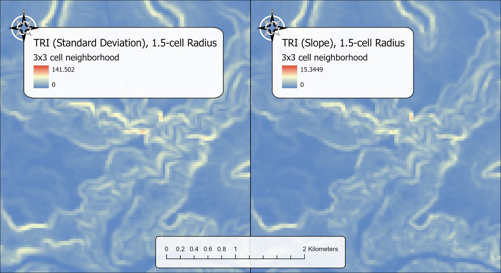
Here the sum runs over all N cells in the neighborhood, focal cell included, and z̄ is their mean. This is the population standard deviation of the elevations, the same number the Focal Statistics tool returns for the Standard Deviation statistic. It measures the spread of the elevations themselves rather than their differences from the center cell, which makes it similar conceptually and mathematically to the Riley index, and nearly identical in pattern (a rank correlation of 0.997 on the Grand Canyon DEM), though about a third the magnitude. For the example, the mean of the nine elevations is 162.8 m and the standard deviation is 19.4 m; compare Riley's 58.7 m, which is a sum over eight cells rather than an average over nine. The output is in the DEM's elevation units.
Reading the four numbers together
Four numbers for one cell: 58.7 m, 17.0 m, 0.459 and 19.4 m. They are not four estimates of one quantity; they are four different quantities, each answering its own question, and that is the difference between this tool and the Fractal Dimension tool, whose methods all estimate the same thing. Choose by the question. If you want to reproduce published work or Riley's classes, use Riley. If you want a stable value across neighborhood sizes and near edges, use Wilson. If the geometry of the diagonals bothers you, or you want a slope-like unitless number, use the slope variant. If you think of ruggedness as the spread of elevations in an area rather than the contrast with its center, use the standard deviation. Whichever you pick, stay with it within a study, and remember that all four rise on a smooth steep slope. That is a feature when a steep even hillside should count as rugged for your species, and a fault when it should not; for the latter case the Vector Ruggedness Measure or the Arc-Chord Ratio is the right tool.
The neighborhood and its scale
The neighborhood is a circle of the radius you set, in cells or in ground units. A radius of 1.5 cells is the classic 3 × 3 window, because the four diagonal neighbors sit about 1.41 cells away and so fall inside 1.5; a radius of exactly 1 cell gives only the four edge neighbors, a plus-shaped neighborhood of five cells. Larger radii measure ruggedness at a coarser landscape scale, and for the Riley and slope methods, which are sums, they also give larger values simply because more neighbors are being added. A radius in meters, kilometers, feet or miles is converted to cells from the cell size, and on a geographic DEM that conversion is done per row on the spheroid so the circle stays the right size at any latitude. The About page discusses choosing a scale; the short version is to try two or three radii and look at what each one shows you.
Missing neighbors are simply ignored. A value is produced wherever the focal cell and at least one neighbor are valid (the same rule applies to the standard deviation), so cells at the raster edge and beside a NoData hole are computed from whatever neighbors they have. Riley et al. do not say how they treated edge cells. The Wilson mean is not pulled down by a partial neighborhood the way the two sums are, which is another reason to prefer it near edges.
A small example shows what a partial neighborhood does to the numbers. Take a perfectly uniform slope that rises 10 m per cell toward the north. Every cell on it is equally rugged, so any change in the index from one cell to the next is purely an effect of the raster edge. A cell in the interior has all eight neighbors; a cell on the east edge of the raster has lost its three eastern neighbors and has five; a cell on the north edge has lost its three northern neighbors and also has five; the cell in the northeast corner only has three neighbors to work with. The cells are 30 m across, which matters only to the slope method.
| Cell on a uniform 10 m-per-cell slope | Neighbors | Riley | Wilson | Slope | Standard deviation |
|---|---|---|---|---|---|
| Interior | 8 | 24.5 m | 7.5 m | 0.667 | 8.2 m |
| East edge | 5 | 20.0 m | 8.0 m | 0.577 | 8.2 m |
| North edge | 5 | 17.3 m | 6.0 m | 0.471 | 5.0 m |
| Northeast corner | 3 | 14.1 m | 6.7 m | 0.408 | 5.0 m |
The Riley index falls at the edges and falls further at the corner, to 82%, 71% and then 58% of its true value, and it can only ever fall: it is a sum of squares, and a missing neighbor is a term left out of the sum. The slope method behaves the same way for the same reason, since it too is a sum of squares, and it falls to 87%, 71% and 61%. The Wilson index wobbles, because the mean is being taken over a different set of neighbors, but it goes up as readily as down: it rises on the east edge, where the three lost neighbors differed from the focal cell by less, on average, than the five that remain, and falls on the north edge, where all three lost neighbors were a full 10 m higher. The standard deviation does something different again. It is a measure of the spread of the elevations in the neighborhood, so what matters is which elevations are lost and not how many. On the east edge the lost column held the same three elevations as the two columns that remain, the spread is unchanged, and the value does not move at all. On the north edge the whole upper row is gone, the neighborhood now spans 10 m of relief where it used to span 20, so in this specific example the value falls to 61%.
To be clear, there is nothing special about north edges or east edges. The difference comes entirely from the fact that this example raster slopes up toward the north: the north edge happens to run across the slope and the east edge happens to run up and down it. Turn the slope to face east and the two edges trade places. The same is true of the Riley, Wilson and slope values in the table.
These edge effects also happen around any NoData hole inside the DEM. They affect only the single ring of cells that touch the edge or the hole at a 1.5-cell radius, and a wider ring at larger radii, so it will not show in a map of a whole landscape; but if your study area runs right to the edge of your DEM and you are using the Riley or slope method, either clip the result back by the radius or extend the DEM beyond the study area before running the tool. (These are the values the tool returns for such a raster.)
A tour of the dialog
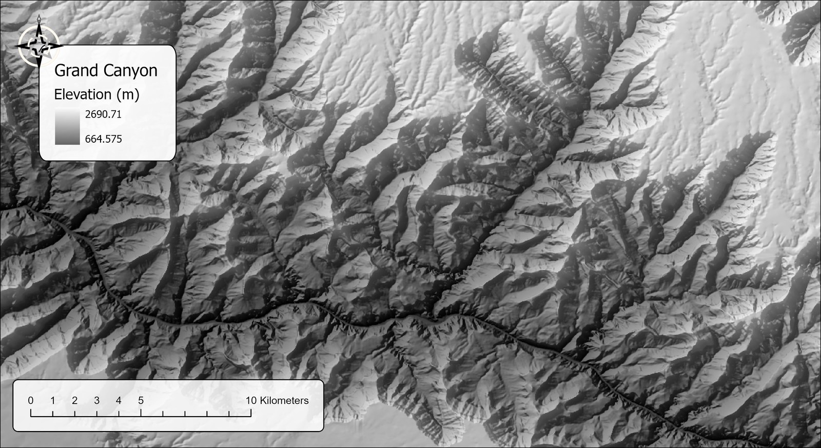
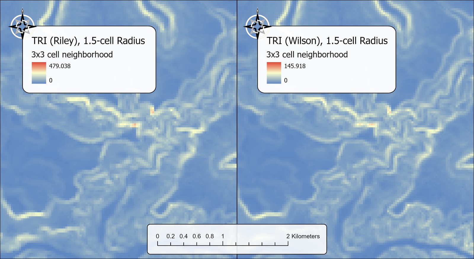
The examples use the same 30 m DEM of the Grand Canyon as the other roughness pages, so the measures can be compared on identical ground. The close-up maps below cover the same 4 km-wide area as the comparison maps on the Arc-Chord Ratio page.
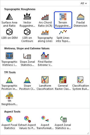
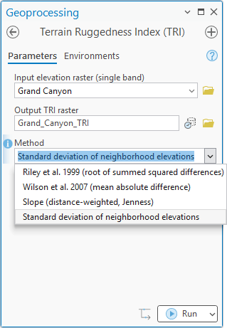
The dialog asks for the DEM, an output name, the method, and the neighborhood radius with its units. An Elevation units row appears only when the tool cannot work the units out for itself, which is why it is absent here. The elevation units serve two purposes. For the Riley, Wilson and standard-deviation methods they only label the output, since those indices are left in whatever units the DEM uses, and the output metadata records which; a DEM in feet gives a result in feet. For the slope method they drive the internal scaling to meters that keeps rise over run dimensionless. The tool reads the units from the DEM's vertical coordinate system and locks the setting when it can, assumes meters for geographic DEMs, and asks you only when the DEM does not say.
What a larger radius does to the numbers
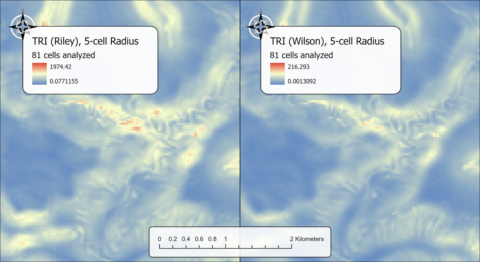
This pair of metrics offers a good demonstration of why you should understand what the method does when you change the radius. When you add more cells to the analysis, you are naturally going to get a larger sum. You won't automatically get a larger mean, though. Across the interior of the DEM, away from its edges, the numbers are these (the raster's legend shows a Wilson maximum of 216 because of one cell on the DEM's edge with only 45 of its 80 neighbors):
| Radius | Neighbors | Riley mean | Riley maximum | Wilson mean | Wilson maximum |
|---|---|---|---|---|---|
| 1.5 cells | 8 | 41.8 m | 479 m | 12.4 m | 146 m |
| 5 cells | 80 | 358 m | 1,974 m | 32.0 m | 184 m |
The Riley mean grew almost ninefold and the Wilson mean grew about two and a half times. The Wilson increase is real terrain: there is more relief within 140 m of a point than within 40 m of it, so the average difference between a cell and its neighbors is larger. The Riley increase is mostly arithmetic. It is the root of a sum, the sum now has 80 terms in it instead of 8, and ten times as many terms would multiply the index by the square root of ten, a little over three, even if the terrain contributed nothing new. A Riley value of 1,974 m does not mean a cell is surrounded by two kilometers of relief (the whole canyon is only about two kilometers deep); it means that eighty squared differences were added together. So if you work at anything other than the 3 × 3 window, either use the Wilson or standard-deviation method, whose values keep their meaning as the neighborhood grows, or treat Riley values as comparable only among runs at exactly the same radius. And Riley's published classes, of course, apply to the 3 × 3 window alone.
The output is a floating-point raster with statistics, a histogram and bilinear pyramids already built, so it draws correctly the moment it reaches the map, with a blue-yellow-red stretch applied by default. Outputs may go into a geodatabase or a folder; in a folder, a name without an extension becomes a GeoTIFF.
The tool holds the whole DEM in memory at once, so the memory it needs grows with the number of cells. On most DEMs that is no concern. On a very large one the tool may need more memory than your computer has free, and then one of two things happens: Windows starts using the disk as overflow memory and the tool slows to a crawl, or the tool stops with an out-of-memory error. There is no fixed limit; it depends on how much memory your computer has free. If a DEM is too large, clip it to the area you need first.
Environment settings
The output matches the input DEM exactly: same extent, cell size and coordinate system. The Processing Extent, Snap Raster, Cell Size, Output Coordinate System and Mask environments are deliberately not applied, so that the delivered raster is the grid the TRI values were computed on; project, clip or resample the finished raster yourself if you need to. Pyramids are always built with bilinear resampling regardless of the Pyramid environment.
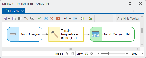
ModelBuilder
Parameters
| Label | Explanation | Data type |
|---|---|---|
| Input elevation raster (single band)Required · in_raster | The DEM. Must be single band; projected or geographic. Choose a layer from the map or browse to a dataset. | Raster Layer |
| Output TRI rasterRequired · out_raster | The ruggedness raster (floating point). In the DEM's elevation units for the Riley, Wilson and standard-deviation methods; a dimensionless rise over run for the slope method. NoData where the focal cell is NoData or has no valid neighbor. A name is suggested from the input. | Raster Dataset |
| MethodRequired · method | Riley et al. 1999 (root of summed squared differences), Wilson et al. 2007 (mean absolute difference), Slope (distance-weighted, Jenness) or Standard deviation of neighborhood elevations, as described above. All four use the neighborhood set below. | String |
| Neighborhood radiusRequired · radius | How far the circular neighborhood extends, in the units below. The default 1.5 cells is the classic 3 × 3 window; 1 cell is the four-neighbor plus; larger radii measure at a coarser scale and, for the sum-based methods, give larger values. The radius is limited to 500 cells (a window about 1,000 cells across); a larger one stops the tool with a message to use a smaller radius or a coarser DEM. | Double |
| Neighborhood radius unitsRequired · radius_units | Cells, Meters, Kilometers, Feet or Miles. Ground units are converted to cells from the cell size, per row on the spheroid for geographic DEMs. | String |
| Elevation unitsOptional · elev_units | Meters or Feet. Filled in and locked from the DEM's vertical coordinate system when it has one; geographic DEMs are assumed to be in meters; you are asked only when the DEM does not say. Labels the output for the three elevation-unit methods and drives the internal scaling for the slope method. | String |
Python
import arcpy
arcpy.ImportToolbox(r"C:\path\to\JennessEnterprisesTools.pyt")  # your install path
# The classic Riley 3 x 3 index.
arcpy.jenness.TRI(
    in_raster=r"C:\Project\Elev.gdb\DEM",
    out_raster=r"C:\Project\Elev.gdb\DEM_TRI_Riley",
    method="Riley et al. 1999 (root of summed squared differences)",
    radius=1.5, radius_units="Cells", elev_units="Meters")
# The slope (distance-weighted) variant at the same 3 x 3 window.
arcpy.jenness.TRI(
    in_raster=r"C:\Project\Elev.gdb\DEM",
    out_raster=r"C:\Project\Elev.gdb\DEM_TRI_Slope",
    method="Slope (distance-weighted, Jenness)",
    radius=1.5, radius_units="Cells", elev_units="Meters")
# Other method strings: "Wilson et al. 2007 (mean absolute difference)",
# "Standard deviation of neighborhood elevations".
Recommended citation
Credits and references
By Jeff Jenness, Jenness Enterprises (www.jennessent.com). The Riley index is the original Terrain Ruggedness Index; the Wilson variant is the mean-absolute-difference form of Wilson et al. (2007); the slope variant and the standard-deviation comparison come from my Topographic Roughness lecture. Riley et al. say of the technique of Beasom et al. (1983), the basis of the LSRI tools, that it “is useful, but laborious if the area of concern is large,” and offer TRI as an easier measure computed from DEMs.
- Beasom, S. L., E. P. Wiggers, and J. R. Giardino. 1983. A technique for assessing land surface ruggedness. Journal of Wildlife Management 47:1163–1166. doi.org/10.2307/3808184
- Jenness, J. Topographic roughness. Lecture, GIS for wildlife and forestry courses, Jenness Enterprises. Slides
- Riley, S. J., S. D. DeGloria, and R. Elliot. 1999. A terrain ruggedness index that quantifies topographic heterogeneity. Intermountain Journal of Sciences 5:23–27. download.osgeo.org/qgis/doc/reference-docs/Terrain_Ruggedness_Index.pdf
- Sappington, J. M., K. M. Longshore, and D. B. Thompson. 2007. Quantifying landscape ruggedness for animal habitat analysis: a case study using bighorn sheep in the Mojave Desert. Journal of Wildlife Management 71:1419–1426. doi.org/10.2193/2005-723
- Valentine, P. C., S. J. Fuller, and L. A. Scully. 2004. Terrain ruggedness analysis and distribution of boulder ridges in the Stellwagen Bank National Marine Sanctuary region (poster). 5th International Symposium on Marine Geological and Biological Habitat Mapping (GeoHAB), Galway, Ireland, May 2004. (As cited by Wilson et al. 2007.)
- Wilson, M. F. J., B. O'Connell, C. Brown, J. C. Guinan, and A. J. Grehan. 2007. Multiscale terrain analysis of multibeam bathymetry data for habitat mapping on the continental slope. Marine Geodesy 30:3–35. doi.org/10.1080/01490410701295962
Licensing information
Works at every ArcGIS Pro license level (Basic, Standard, Advanced). No extension licenses are required; the neighborhood statistics are computed internally, without Spatial Analyst.
Related tools and pages
- About Topographic Roughness — choosing among the nine roughness measures, and the three generations of ruggedness index.
- Vector Ruggedness Measure (VRM) — the slope-independent alternative: variation in the direction cells face.
- Arc-Chord Ratio (ACR) — surface roughness with the tilt removed.
- Surface Area and Ratio — the same worked-example cell, as surface area.
- Fractal Dimension — roughness across scales rather than at one neighborhood size.
- LSRI on DEM — the contour-length index that TRI was built to automate.
- Projecting Rasters — this tool works on geographic DEMs directly; if you project a DEM first, use bilinear interpolation.