

LSRI on DEM
Summary
Computes the Land Surface Ruggedness Index (LSRI) of Beasom, Wiggers and Giardino (1983) directly from a DEM: the total length of contour line within a circular neighborhood of every cell. Contours are traced from the DEM on the fly, with the same contour interval, base contour and z-factor logic as Esri's Contour tool and no smoothing, and the tool then measures exactly how much of that contour line falls inside the circle around each cell. Higher values mean more contour line nearby, or more convoluted contour line, which is to say more rugged terrain. The derived contours can be saved for inspection or reuse, and the output can be computed on a coarser grid than the DEM to save time on very large rasters. Correct on geographic (latitude/longitude) DEMs. No Spatial Analyst or 3D Analyst license is needed.
Contour lines as a measure of ruggedness
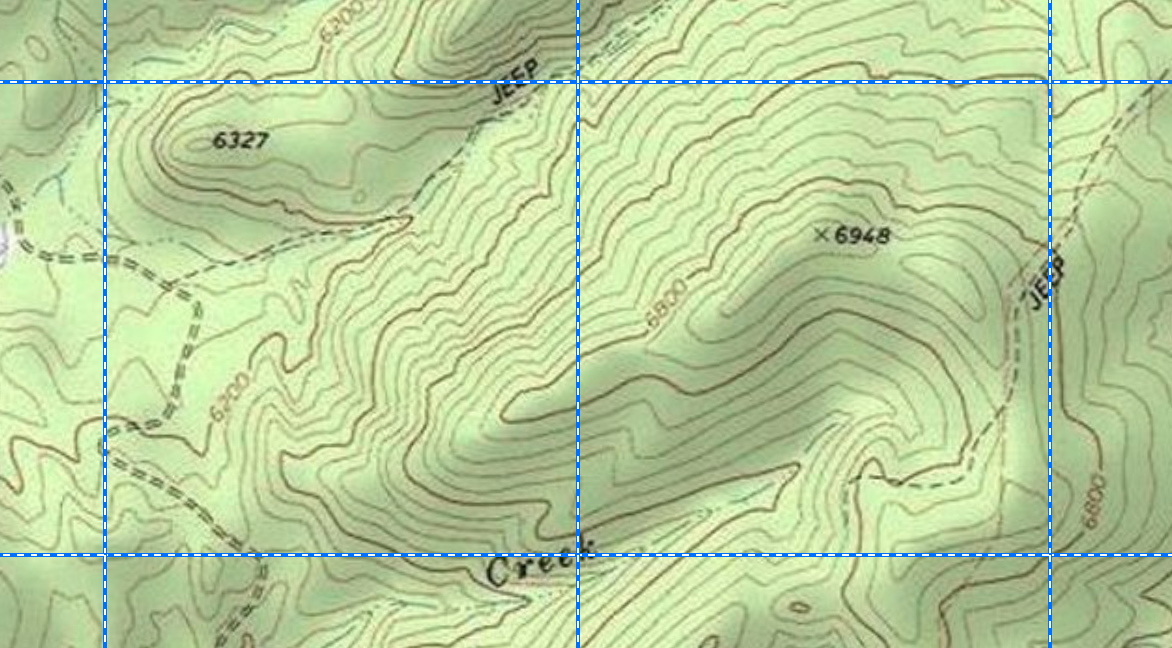
Anyone who has read a topographic map has an instinct for this one. Where the contour lines crowd together the ground is steep, and where they wiggle in and out of every gully the ground is broken. Beasom, Wiggers and Giardino (1983) turned that instinct into an index. Their basic assumption was that ruggedness is a function of the total length of all the contour lines crossing a given area, and total length rises with two things at once: the number of contour lines, which reflects the elevation change across the area, and the irregularity of each line, which reflects how dissected the surface is. A smooth steep slope has many nearly straight contours; a broken steep slope has many convoluted ones; a plain has almost none.
They tested the assumption on three 40-hectare circular areas chosen by eye from three-dimensional maps to represent rugged, rolling and level terrain, on 7.5-minute USGS maps with 3.04 m (10 ft) contour intervals. Running a tracing wheel along every contour from where it entered the circle to where it left, they measured 486 cm of contour line in the rugged area, 178 cm in the rolling one and 8 cm in the level one. That is a sixty-fold range across three areas of identical size, and it matched the visual ranking exactly. Total contour length, measured directly, was the accurate assessment of ruggedness.
Tracing every contour line with a wheel, however, is slow, and they wanted to classify many areas. So for the main study they substituted a dot grid: a circle of transparent plastic representing 40 hectares at the map scale, with 96 uniformly spaced dots on it, laid over each of 80 further areas chosen to span a wide range of terrain (69 in west Texas and 11 in central Colorado). The number of dots landing on a contour line was recorded as the Land Surface Ruggedness Index for that area, and total contour length was also measured on each. LSRI ranged from 0 to 244 and contour length from 4 to 521 cm, and the two were tightly related (length = 5.92 + 1.52 × LSRI, r = 0.93). The dot count was a proxy for contour length, in other words, and a good one; the quantity it stood in for was always the length.
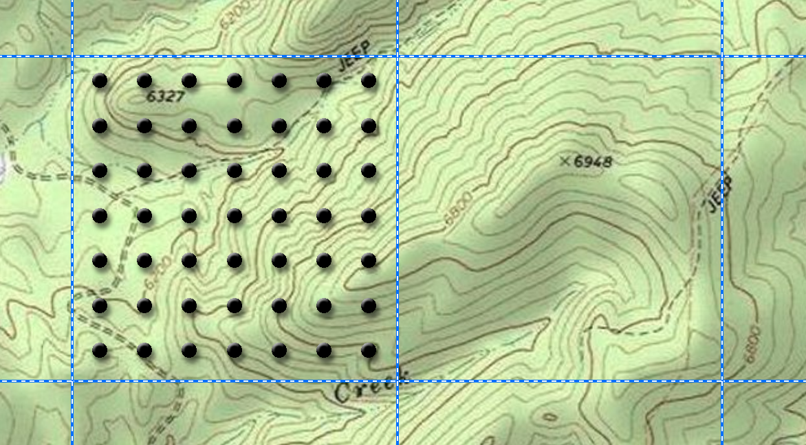
This tool automates the length measurement, which was the more accurate of their two methods, and applies it not to one fixed circle per plot but to a moving circle centered on every cell of the output raster, so what you get is a continuous ruggedness surface rather than one number per plot.
LSRI was, as Sappington et al. (2007) put it, the first widely recognized method for quantifying ruggedness among biologists, and, they note, it or variations of it have been used in a wide variety of habitat analyses. It is a first-generation index in the terms of Dilts et al. (2023): it responds to slope as well as to brokenness, because a steep smooth hillside genuinely does hold more contour line than a plain. If that is what you mean by rugged, it is exactly the right measure; if you want a measure that ignores steepness, see the Vector Ruggedness Measure.
The contour interval matters, exactly as you would expect
The three contour intervals on Beasom's maps (3.04, 6.10 and 12.19 m) gave them a problem that you will have too: an area drawn with a 6.10 m interval has about half as many contour lines as the same area drawn with a 3.04 m interval, so its LSRI should be about half as large. They tested this by re-counting 30 of the 3.04 m areas using only every other contour line, and a chi-square test found no departure from the expected 2:1 ratio. They therefore standardized every value to the 3.04 m interval, multiplying the 6.10 m readings by 2 and the 12.19 m readings by 4.
The same rule applies to this tool. Halve the contour interval and LSRI roughly doubles wherever the relief crosses several contours, because every slope now needs twice as many lines to describe it. Suppose, as a made-up example, that a cell's neighborhood holds 1,840 m of contour line at a 20 m interval; at a 10 m interval it would hold something close to 3,680 m, and at 5 m something close to 7,360 m. The relationship is only approximate on real terrain, because the extra lines fall in different places, and it is variable enough that you must never compare LSRI values computed at different intervals. Pick an interval, keep it for every run in a study, and report it with your results. A smaller interval sees finer relief and gives larger numbers; the interval is not a scale control so much as a units control, and the neighborhood radius (below) is where you set the scale.
What the tool measures
The tool does three things. First it generates contour lines from the DEM. Second it breaks those lines into straight segments. Third, for every cell of the output raster, it draws a circle of the chosen radius around the cell center and adds up the exact length of contour line that lies inside the circle. That sum, converted to the length units you chose, is the cell's LSRI.
Generating the contours
The contours are traced by the same rule as Esri's Contour tool, and the three parameters mean the same things. The contour interval is the vertical distance between lines, in the DEM's elevation units. The base contour is the elevation the lines are counted from; with a base of 10 and an interval of 15, the contours fall at 10, 25, 40, 55 and so on, and lines are generated above and below the base as needed to cover the DEM's full range. The z factor multiplies the elevations before contouring, so that a DEM in feet can be contoured at a 10 m interval by setting the z factor to 0.3048. In development testing on a synthetic cone-shaped DEM, the contour levels came out exactly at Esri's documented base-plus-interval values, and the length of each interior contour matched the true circumference of its circle to about 0.01%.
The contours are deliberately not smoothed. Esri's Contour tool offers no smoothing option either, and the reason it matters here is that smoothing would shorten exactly the wiggles this index exists to measure. A contour that follows every side gully has length because of those gullies; smooth it and the ruggedness goes down while the terrain stays the same. The raw contour follows the cell grid, and that is what the tool measures. Turn on Save the contour feature class if you want to see the lines the tool used, or to feed them to LSRI on Contours later without contouring again.
Measuring length inside the circle exactly
This is the part I want to explain carefully, because it is what makes the number an exact length rather than an approximation. Every contour line is a chain of straight segments. For a given cell center C and radius r, a segment from point P0 to point P1 may lie entirely inside the circle, entirely outside it, or partly inside. The tool finds the exact portion inside by writing the segment as P(t) = P0 + t(P1 − P0) for t from 0 to 1, and solving for the two values of t where the segment crosses the circle:
where d = P1 − P0 is the segment vector and f = P0 − C runs from the center to the segment's start. The three coefficients come from nothing more than expanding the left side. P(t) − C is f + t d, and the squared length of a vector is the vector dotted with itself, so
Moving r² to the left gives a = |d|², b = 2 f·d and c = |f|² − r². This is the standard way of intersecting a line with a circle or a sphere, the same calculation a ray tracer does, and the tool's code does it in exactly these terms. The quadratic formula gives the two crossing values t1 and t2; clipping both to the range 0 to 1 keeps only the part of the segment that actually exists; and the length inside the circle is (t2 − t1) times the segment's full length. If the discriminant is negative the segment misses the circle entirely and contributes nothing. For a segment that passes right through, this reduces to the familiar chord length:
where h is the perpendicular distance from the center to the line. Two examples, both with a 200 m radius and a horizontal contour segment passing 100 m north of the cell center. First, a long segment running from 300 m west of center to 300 m east: d = (600, 0), f = (−300, 100), so a = |d|² = 600² = 360,000; b = 2 f·d = 2 × (−300 × 600 + 100 × 0) = −360,000; and c = |f|² − r² = (300² + 100²) − 200² = (90,000 + 10,000) − 40,000 = 60,000. The roots are t = 0.211 and t = 0.789, both inside 0 to 1, so the segment spans the circle and contributes (0.789 − 0.211) × 600 = 346.4 m. That is the chord: 2 × √(200² − 100²) = 346.4 m. Second, a shorter segment running from 100 m west of center to 200 m east: d = (300, 0), f = (−100, 100), a = 90,000, b = −60,000, c = (10,000 + 10,000) − 40,000 = −20,000, and the roots are t = −0.244 and t = 0.911. The first root falls before the segment starts and is clipped to 0; the segment therefore begins inside the circle, and it contributes (0.911 − 0) × 300 = 273.2 m. You can check that by hand too: the circle crosses the line 100 m north of center at 173.2 m east, so the inside portion runs from −100 m to +173.2 m, which is 273.2 m. The chord formula would have overstated this segment by 73 m; the general solution gets it right.
This calculation is done for every combination of output cell and nearby contour segment, which on a large DEM can be billions of pairs, so the tool organizes the work carefully: the segments are indexed in a spatial tree, only the segments that could possibly touch each circle are examined, and the work is done in bounded blocks, several at a time on separate processor cores, so memory stays under control however many contours a fine interval on a rugged DEM produces, up to a limit: a run stops with an error above 5,000,000 contour segments, or 20,000,000 of the pieces they are subdivided into, and the remedy is a larger contour interval or a smaller processing extent. None of that changes the arithmetic; it just keeps the run from exhausting your computer. The progress bar reports the share of those pairs completed and an estimate of the time remaining, and the run messages report how many pairs there were. The engine was validated against Esri's Line Density tool on a controlled test with a straight line and a zigzag line 28 times longer, and the lengths matched the true values to full floating-point precision.
Esri's Line Density tool is the natural point of comparison, since it also measures linear features within a circular neighborhood of each cell. The two differ in what they report: Line Density divides the length by the circle's area to give a density (length per unit area), whereas this tool reports the total length itself, which is Beasom et al.'s original quantity. Since every cell uses the same circle, the two are proportional within one run, but the length is what Sappington et al. (2007) computed as LSRI, and the length is what you get here. The tool computes it independently with its own exact clipping; it does not run Line Density internally.
Choosing the radius
The neighborhood radius is the scale of the analysis, and there is no default because there is no universal right answer. Beasom et al. used 40-hectare circles, which is a radius of about 356.8 m, and I mention the figure for anyone who wants to reproduce their scale. Beasom et al. do not say why they chose 40 hectares; it may have just been a practical size to trace by hand on a printed 7.5-minute map. If so, that is a paper-map constraint, not an ecological one, and a computed neighborhood is free of it. Sappington et al. (2007), working on bighorn sheep with 30 m DEMs, measured LSRI in a 90 × 90 m box instead. Think about the organism and the question: a radius of a few cells describes ruggedness underfoot, a radius of a kilometer describes the ruggedness of a mountain front, and both are legitimate. Also, as with many circular neighborhood-based analyses, it is difficult to know what the best radius to use is. We never have enough information to know exactly, so it is not uncommon to try multiple radii until you get something that looks reasonable and defensible to you; the About page has more on why. A larger radius always gives larger values, simply because a bigger circle holds more line, so, as with the contour interval, compare runs only at the same radius.
The radius may be given in cells, meters, kilometers, feet or miles. In cells it is sized from the DEM's own cell size; in ground units it is converted to the DEM's map units. On a geographic DEM, a ground-unit radius is exact and the Cells unit uses one representative ground cell size, taken at the DEM's central row, since a degree of longitude is a different number of meters at each latitude.
Geographic DEMs
The tool accepts DEMs in geographic (latitude/longitude) coordinate systems directly, and this is worth a paragraph because a naive implementation would get it badly wrong. A degree of latitude is about 111 km everywhere, but a degree of longitude shrinks from 111 km at the equator to 79 km at 45° and to nothing at the poles, so a circle drawn in degrees is an ellipse on the ground and a length measured in degrees is not a length at all. This tool converts every contour vertex and every cell center to three-dimensional Earth-centered coordinates on the DEM's own reference spheroid, in meters, and runs the circle clip in that space. The neighborhood is then a true ground circle and the lengths are true ground lengths at any latitude, including near the poles. The chord distance through the Earth differs from the distance along its surface by about a millimeter at a 10 km radius, so the approximation is negligible. There is no need to project the DEM first, which spares it the resampling that projection imposes (see Projecting Rasters).
Output cell size and run time
By default the output raster has the DEM's cell size, so every DEM cell gets its own LSRI value. On a large, fine-resolution DEM that can be slow, and the reason is instructive: the contour tracing is quick, and what scales the run time is the number of output cells, each of which needs its own circle clip against every nearby segment. The Output cell size parameter lets you compute the index on a coarser grid, in the DEM's map units, while the contours are still traced at the DEM's full native resolution. Accuracy is unaffected; you are only choosing how many places to evaluate the index. For a 3-million-cell DEM, evaluating at three times the cell size cuts the number of output cells, and roughly the run time, by a factor of nine. Whether a 90 m grid is fine enough is a judgment about your question; the accuracy of each value is unchanged. The Grand Canyon DEM in the examples below, 2 million cells at a 10 m interval over 2,000 m of relief, produced 4.2 million contour segments and 4.6 billion segment-to-cell comparisons at a 500 m radius, which took about four minutes on eight processor cores. Because run time scales with the number of output cells, a coarser output cell size is the most direct way to shorten a run like that.
A tour of the dialog
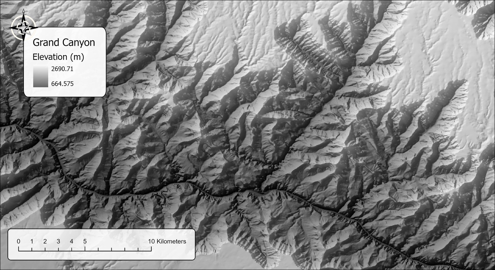
The examples use the same 1-arc-second DEM of the Grand Canyon as the other pages in this group (geographic coordinates; cells about 25 m east–west by 31 m north–south), so the results can be compared with the other indices over identical ground.
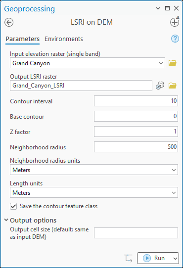
The dialog opens with the DEM and the output raster name, then the three contouring parameters, then the radius and its units, then the length units for the output values, then the checkbox and feature class name for saving the derived contours. Under Output options is the output cell size, blank by default; a blank output cell size means the output matches the DEM. The contour interval, base contour, Z factor, radius and both unit choices are remembered from the last run. The radius has no default the first time, and its units start at Meters.
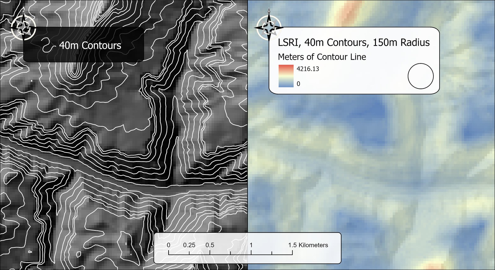
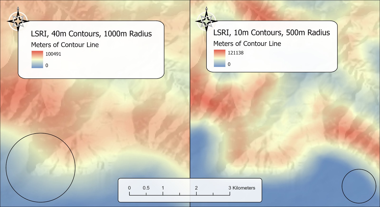
The output is a floating-point raster whose values are lengths in the chosen units. A cell whose circle contains no contour line at all, such as the middle of a flat valley, is 0, and the values climb from there; there is no upper bound, and typical magnitudes depend entirely on the interval and radius. Cells are NoData where the DEM is NoData. The raster carries statistics, a histogram and pyramids so it draws correctly at once, with the same blue-yellow-red stretch the other roughness tools use. As with every tool in this group, a folder output without an extension becomes a GeoTIFF.
Cells within one radius of the DEM's edge, or of a NoData gap, have circles that reach where there are no contours at all, so their values run low. The output grid is the DEM grid, and there is no correction for this: read the outer ring, one radius wide, as an edge artifact, or run the tool on a DEM that extends one radius beyond the area of interest.
The tool holds the whole DEM in memory at once, so the memory it needs grows with the number of cells. On most DEMs that is no concern. On a very large one the tool may need more memory than your computer has free, and then one of two things happens: Windows starts using the disk as overflow memory and the tool slows to a crawl, or the tool stops with an out-of-memory error. There is no fixed limit; it depends on how much memory your computer has free. If a DEM is too large, clip it to the area you need first.
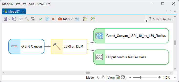
ModelBuilder
Parameters
| Label | Explanation | Data type |
|---|---|---|
| Input elevation raster (single band)Required · in_raster | The DEM to contour and compute LSRI from. Must be single band; projected or geographic. | Raster Layer |
| Output LSRI rasterRequired · out_raster | The total length of contour line within the neighborhood radius of each cell, in the length units. Floating point. A name is suggested from the input. | Raster Dataset |
| Contour intervalRequired · contour_interval | The vertical distance between contour lines, in the DEM's elevation units (or in the units the z factor converts them to). A smaller interval means more lines and a higher LSRI; compare runs only at the same interval. | Double |
| Base contourOptional · base_contour | The elevation the contours are counted from; default 0. Base 10 with interval 15 gives 10, 25, 40, 55 and so on. Lines are still generated above and below it as needed. | Double |
| Z factorOptional · z_factor | Multiplies the elevations before contouring; default 1. Use 0.3048 to contour a DEM in feet at a metric interval. | Double |
| Neighborhood radiusRequired · radius | How far the circle extends around each cell, in the radius units. No default: choose the scale that suits your question. Beasom et al.'s 40 ha circle is about 356.8 m if you want their scale. Larger radii give larger values. | Double |
| Neighborhood radius unitsRequired · radius_units | Cells (sized from the DEM's cell size), Meters, Kilometers, Feet or Miles (converted to the DEM's map units; exact on geographic DEMs). | String |
| Length unitsOptional · length_units | The units of the output values: Meters (default), Feet, Kilometers or Miles. | String |
| Output cell size (default: same as input DEM)Optional · out_cell_size | The cell size of the output raster in the DEM's map units; blank matches the DEM. Contours are always traced at the DEM's native resolution, so a coarser value trades nothing but output detail for a large saving in run time. | Double |
| Save the contour feature classOptional · save_contours | Check to save the contour polylines the tool generated, unsmoothed, with one attribute, a Contour field holding each line's elevation, for inspection or for reuse with LSRI on Contours. | Boolean |
| Output contour feature classOptional · out_contours | Where to save the contours. Used only when the box above is checked. | Feature Class |
Python
import arcpy
arcpy.ImportToolbox(r"C:\path\to\JennessEnterprisesTools.pyt")  # your install path
# LSRI with a 10 m contour interval and a 500 m neighborhood, saving the contours.
arcpy.jenness.LSRIOnDEM(
    in_raster=r"C:\Project\Elev.gdb\DEM",
    out_raster=r"C:\Project\Elev.gdb\DEM_LSRI",
    contour_interval=10, base_contour=0, z_factor=1,
    radius=500, radius_units="Meters", length_units="Meters",
    save_contours=True,
    out_contours=r"C:\Project\Elev.gdb\DEM_Contours")
# The same index evaluated on a 90 m output grid to cut the run time.
arcpy.jenness.LSRIOnDEM(
    in_raster=r"C:\Project\Elev.gdb\DEM",
    out_raster=r"C:\Project\Elev.gdb\DEM_LSRI_90m",
    contour_interval=10, radius=500, radius_units="Meters",
    length_units="Meters", out_cell_size=90)
Recommended citation
Credits and references
By Jeff Jenness, Jenness Enterprises (www.jennessent.com), automating the contour-length measurement of Beasom, Wiggers and Giardino (1983) over a moving neighborhood. The contour tracing follows the interval, base and z-factor conventions of Esri's Contour tool.
- Beasom, S. L., E. P. Wiggers, and J. R. Giardino. 1983. A technique for assessing land surface ruggedness. Journal of Wildlife Management 47:1163–1166. doi.org/10.2307/3808184
- Dilts, T. E., M. E. Blum, K. T. Shoemaker, P. J. Weisberg, and K. M. Stewart. 2023. Improved topographic ruggedness indices more accurately model fine-scale ecological patterns. Landscape Ecology 38:1395–1410. doi.org/10.1007/s10980-023-01646-6
- Esri. Contour (Spatial Analyst) tool reference, ArcGIS Pro. pro.arcgis.com/.../spatial-analyst/contour.htm. Accessed on 28 September 2026.
- Esri. Line Density (Spatial Analyst) tool reference, ArcGIS Pro. pro.arcgis.com/.../spatial-analyst/line-density.htm. Accessed on 28 September 2026.
- Jenness, J. Topographic roughness. Lecture, GIS for wildlife and forestry courses, Jenness Enterprises. Slides
- Riley, S. J., S. D. DeGloria, and R. Elliot. 1999. A terrain ruggedness index that quantifies topographic heterogeneity. Intermountain Journal of Sciences 5:23–27. download.osgeo.org/qgis/doc/reference-docs/Terrain_Ruggedness_Index.pdf
- Sappington, J. M., K. M. Longshore, and D. B. Thompson. 2007. Quantifying landscape ruggedness for animal habitat analysis: a case study using bighorn sheep in the Mojave Desert. Journal of Wildlife Management 71:1419–1426. doi.org/10.2193/2005-723
Licensing information
Works at every ArcGIS Pro license level (Basic, Standard, Advanced). No extension licenses are required; the contours are traced and the lengths measured internally, without Spatial Analyst or 3D Analyst.
Related tools and pages
- About Topographic Roughness — choosing among the nine roughness measures.
- LSRI on Contours — the same index from contour lines, or any polylines, you already have.
- Terrain Ruggedness Index (TRI) — the other classic first-generation index (Riley et al. 1999), from elevation differences instead of contour length.
- Vector Ruggedness Measure (VRM) — ruggedness independent of slope.
- Surface Area and Ratio — roughness as extra land surface.
- Projecting Rasters — why geographic DEMs can be used directly, and how to project one properly when you must.