

About Topographic Position Index
What it is for
The Topographic Position Index is an automated way to identify and classify topographic features, such as hills, valleys, ridges, canyons and plains, according to their height relative to the landscape around them. It needs nothing but a DEM, it is repeatable, and it turns a continuous surface of elevations into the kinds of features that people, and the animals and plants they study, respond to. Weiss (2001) lists the reasons those features matter: soil erosion and deposition, hydrologic balance and response, wind exposure, and cold-air drainage all follow topographic position, and through them so do habitat suitability, community composition, and the distribution and abundance of species. In wildlife work the index has been used to describe how cougars move through a landscape (Dickson and Beier 2007), to build the topographic position factor of a habitat suitability model, and to partition a landscape into canyons, slopes and ridges before defining land facets; in geomorphology, to map landforms across a whole watershed (Tağıl and Jenness 2008).
The catch is that a hill is in the eye of the beholder. What is a hill to a mouse is a ripple to a bighorn or a cougar, and what a road construction crew calls a ridgetop may be a flat plain to the mouse living on it. The same crest of a mountain range is all of these things at once, and none of them is wrong. The index deals with this honestly: it measures height relative to a neighborhood of a chosen size, and the size of that neighborhood is the scale at which the landscape is being read. Choosing it is the analyst's first and most consequential decision, and most of this page is about how to make it.
What the index is
The Topographic Position Index (TPI) is the difference between the elevation of a cell and the mean elevation of a neighborhood around it (Weiss 2001, after Guisan et al. 1999):
where z0 is the elevation of the cell and z̄ is the mean elevation of the cells in its neighborhood. A positive value means the cell stands above its surroundings, as on a ridge or hilltop; a negative value means it sits below them, as in a valley or channel. A value near zero means only that the cell is at about the mean elevation of its neighborhood, which is true both of a flat plain and of an even mid-slope, so slope is used to tell the two apart: near-zero TPI with a gentle slope is a flat, and near-zero TPI with a steep slope is somewhere on the side of a hill.
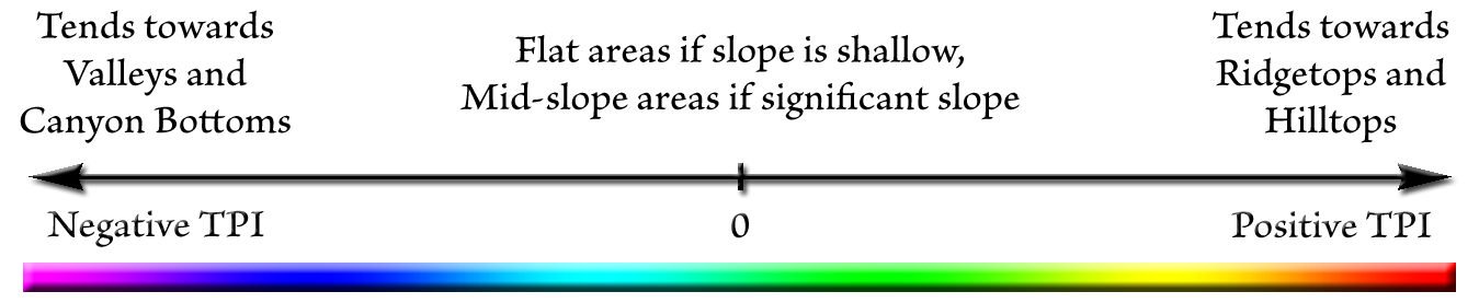
Weiss presented the index, and the slope-position and landform classifications built on it, in a poster at the 2001 ESRI International User Conference, as part of work for the EPA's western landscape assessment (Jones et al. 2000). The index itself had been used earlier in species-distribution modeling in the Spring Mountains of Nevada (Guisan et al. 1999). The only input it needs is a DEM, so it can be computed almost anywhere, and the tools on this site compute it, and everything derived from it, with no Spatial Analyst license.
Scale is part of the answer
TPI is a scale-dependent quantity, and the neighborhood is the scale. Weiss's poster gives the example of a meadow in Yosemite Valley: at a scale of 100 m it is a flat plain, which may be the right scale for questions of soil transport or site water balance; at a scale of several kilometers the same point is the bottom of a 1,500 m canyon, which matters more for hydrology, mesoclimate, wind exposure and cold-air drainage.
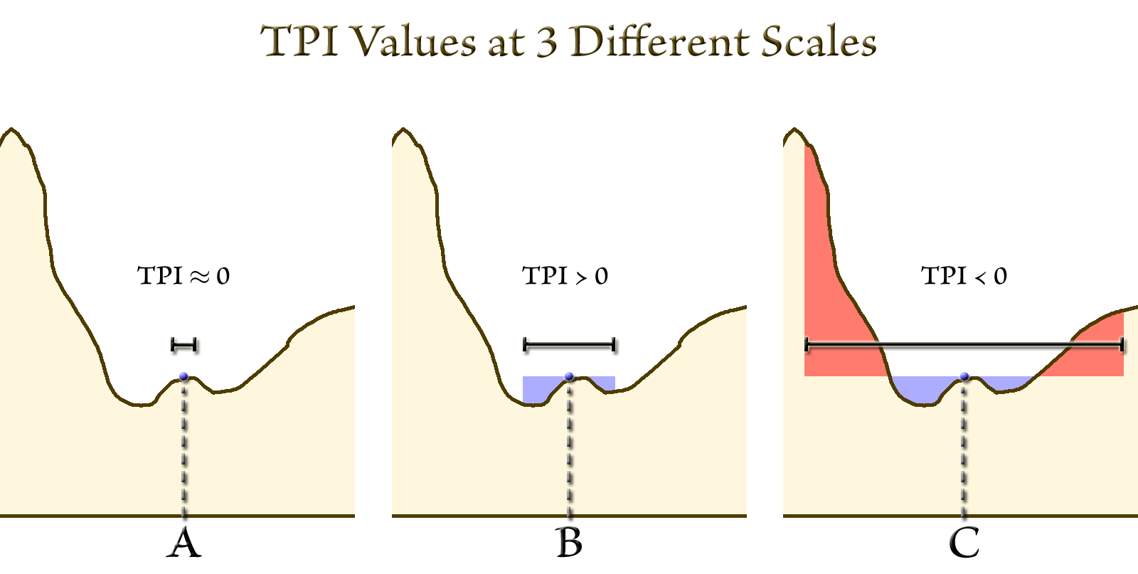
All three answers are correct. A point on top of a small hill at the bottom of a canyon is a hilltop at one scale and a canyon bottom at another, and the analyst has to decide which scale is relevant to the question. For the topographic habitat of a large, wide-ranging animal, the classes should be defined in terms of large, distinctive features: a cougar is likely to be influenced far more by a ridgeline hundreds of feet high than by the minor ripples and bumps immediately around it, so a large neighborhood is the right choice. For soil, small plants or surface water, a small one is. In the Spring Mountains study, Guisan et al. (1999) computed the index at four radii, 150, 300, 1,000 and 2,000 m, and offered all four to regression models of 22 plant species. Elevation entered 21 of the models; topographic position at 300, 1,000 or 2,000 m entered 17, the same number as the insolation and northness variables, and the 150 m index entered none. Different species picked different scales, so the ecological characteristics of a site can depend on TPI at several scales at once.
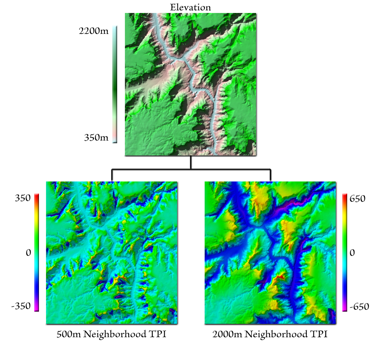
The neighborhood defines which cells count as being “around” a cell. A circle takes every cell within a radius; an annulus, the shape Weiss's own examples used, takes only the ring of cells between an inner and an outer radius. On his 30 m DEM the 300 m index used an annulus from 5 to 10 cells and the 2,000 m index an annulus from 62 to 67 cells. Rectangular neighborhoods are used by some researchers, though a circle or annulus is usually the more reasonable choice for ecological analysis, and Weiss proposed wedge-shaped, directional neighborhoods as future work, to separate saddles from flats and ridges from hilltops. The tools here offer circles and annuli, with the radius in cells or in ground units. A cell is in the neighborhood when its center lies within the radius and not otherwise. On a geographic (latitude/longitude) DEM a ground-unit radius is worked out per row on the spheroid, since a degree of longitude shrinks toward the poles; for the neighborhood mean and standard deviation the east-west radius is then rounded to a whole number of cells for each band of rows (the percentile uses the exact value), so the neighborhood is a circle on the ground to within about half a cell east-west at any latitude. One practical point from the Yazoren study below: cells near the edge of a DEM have incomplete neighborhoods, so it pays to run the analysis on an area larger than the study area, by at least the neighborhood radius, and clip afterward.
Slope position: one scale plus slope
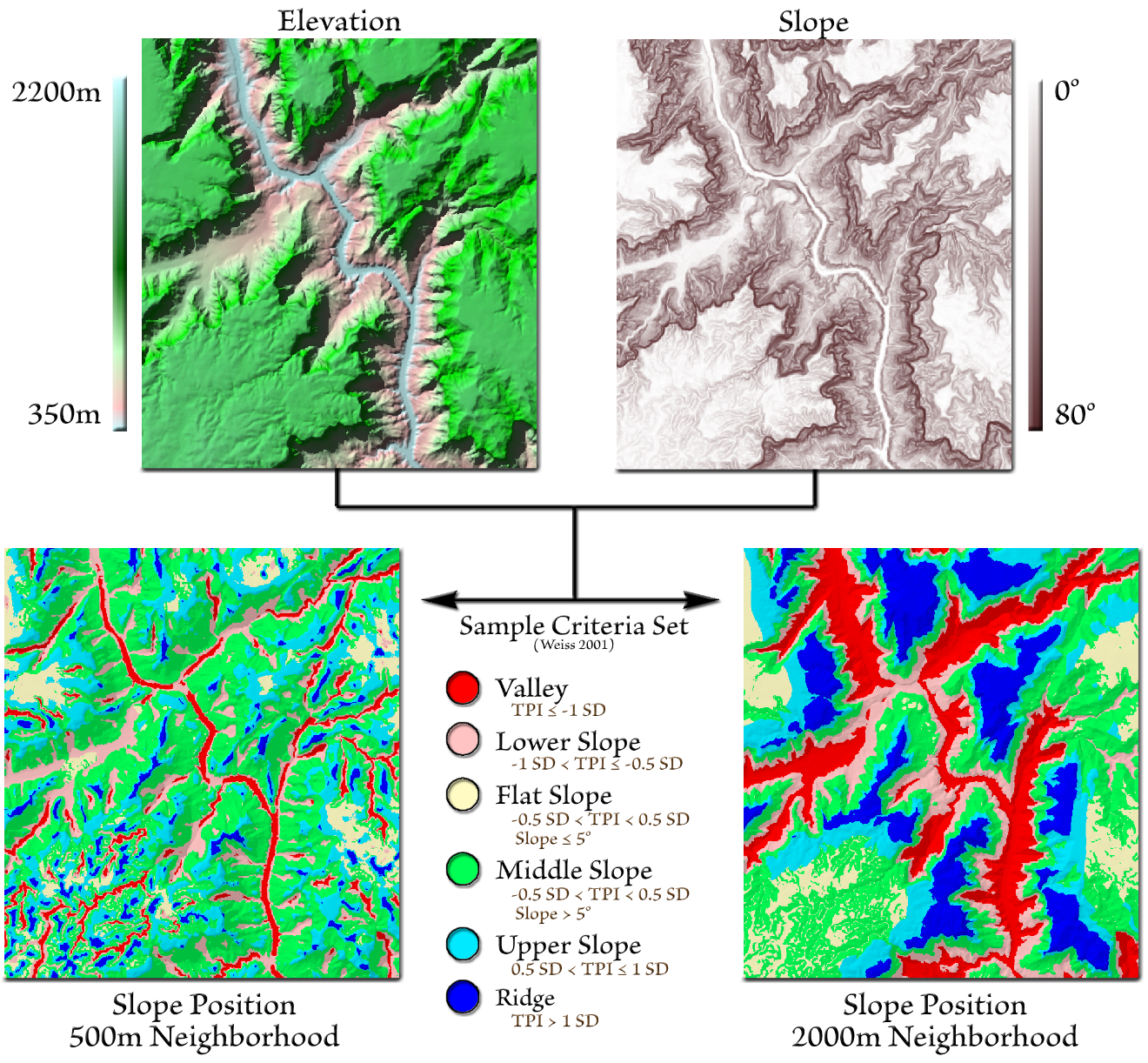
Because high TPI means a hilltop or ridge, low TPI means a valley bottom, and near-zero TPI means a flat or a mid-slope depending on the slope, a single TPI raster plus a slope raster can be thresholded into slope-position classes. Weiss's poster illustrates a six-class scheme: valley, lower slope, flat, middle slope, upper slope and ridge.
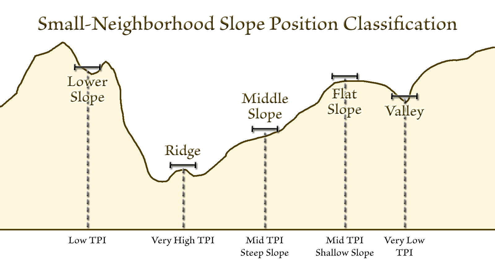
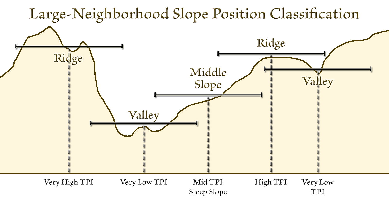
Weiss's six-class scheme sets its TPI thresholds in standard-deviation units, which the next section explains. The system bundled with the Slope Position Classification tool is adapted from that scheme; its classes are:
| Class | TPI (standard-deviation units) | Slope |
|---|---|---|
| Valley | TPI ≤ −1 | |
| Lower slope | −1 < TPI ≤ −0.5 | |
| Flat slope | −0.5 < TPI < 0.5 | ≤ 5° |
| Middle slope | −0.5 < TPI < 0.5 | > 5° |
| Upper slope | 0.5 ≤ TPI ≤ 1 | |
| Ridge | TPI > 1 |
Simpler schemes set their thresholds directly in elevation units. Dickson and Beier (2007), studying how topographic position influences cougar movement in southern California, used four classes: ridgeline where TPI ≥ 8, canyon bottom where TPI ≤ −8, and the ground between split at a 6° slope into gentle and steep slope. The CorridorDesigner toolbox (Majka et al. 2007) used the same shape with wider thresholds for its topographic-position habitat factor: canyon bottom at TPI ≤ −12, ridgetop at TPI ≥ 12, and flat-gentle versus steep slope split at 6°, with the TPI computed over a 200 m circular neighborhood. The land facet method (Beier and Brost 2010; Brost and Beier 2012) needed only three classes, canyons, slopes and ridges, to partition a landscape before clustering it into land facets; in the Land Facet Corridor Designer, Jenness, Brost and Beier (2013) experimented with neighborhood sizes in three landscapes and settled on a radius of 5 cells with raw TPI thresholds of −6 and +6 m, while advising users to experiment in their own landscapes. All four systems ship with the Slope Position Classification tool, and the Classification System Builder page builds the three-class scheme step by step as its worked example.
Raw versus standardized
TPI thresholds can be set in two very different ways, and the choice decides what the classes mean.
Raw TPI is in the DEM's elevation units. A threshold is then absolute relief: a cell 100 m above its neighborhood mean reads as +100 wherever it occurs, in the mountains or on a plain. This is usually the appropriate form for ecological and wildlife questions, where what an animal experiences is the actual height of the ridge or depth of the canyon, and it is the form Dickson and Beier (2007) used. Its cost is that the thresholds have to be chosen for the landscape at hand, as Weiss (2001) put it: a ridge in Kansas is different from a ridge in central Colorado.
Standardized TPI expresses the value relative to the variability of the terrain, so the thresholds are dimensionless and can be carried from one landscape to another. The bundled systems adapted from Weiss divide each cell's TPI by the standard deviation of the elevations within that cell's neighborhood, so the threshold “1 standard deviation” means one standard deviation of the local relief. (Weiss's poster standardized differently, converting each whole TPI raster to z-scores; see Landforms from two scales below.) The consequence is that cells with identical raw TPI can land in different classes in different parts of the map: a cell must clear a higher bar where its surroundings are more variable. A 1 m rise on a plain and a 100 m rise in the mountains can fall in the same class. That is useful when a classification must adapt to each landscape or be comparable across very different terrains, and misleading when absolute relief is what the question is about.
The Topographic Position Index tool offers five forms of the index, and the classification systems record which form their thresholds assume:
- TPI in elevation units, the raw index; the “diff” statistic of Wilson and Gallant (2000, equation 3.27).
- TPI standardized at neighborhood scale, the raw TPI divided by the standard deviation of elevation within the cell's own neighborhood; Wilson and Gallant's “dev” (equation 3.30), and the form used by the bundled six-class and ten-class systems adapted from Weiss.
- TPI in percentile units, the percentage of the neighborhood's cells that are lower than the cell, from 0 for the lowest cell in its neighborhood upward. Because the cell itself is counted among the neighborhood's n cells, the highest cell in a circle scores 100(n − 1)/n rather than 100: 88.9 in a 9-cell circle, and above 99 once the circle holds more than 100 cells. A percentile class such as Ridge in the bundled percentile system, above 90, therefore cannot occur with a radius under 2 cells, and the classification tools warn whenever a percentile class threshold cannot be reached with the neighborhood used. This is Wilson and Gallant's “pctl” (equation 3.31). It is a rank rather than a distance, so it is untroubled by the units of the DEM.
- TPI standardized at DEM scale, the cell's elevation minus the mean elevation of the whole DEM, divided by the standard deviation of the whole DEM. This is independent of any neighborhood: it says how high the cell sits within the DEM's elevation distribution, not how it sits relative to its surroundings, so it is offered for completeness rather than for classification.
- An experimental form, the raw TPI divided by the standard deviation of the TPI values in the neighborhood, which measures position relative to the local roughness of the terrain-position surface rather than the local relief. It is numerically unstable on smooth slopes, where both numerator and denominator approach zero, and for that reason it is not offered to the classification tools.
Two older forms deserve a word because they appear in earlier versions of these tools and in the literature. The ArcView extension and the ArcMap Land Facet Corridor Designer tools offered a “standardized TPI” that subtracted the mean TPI of the whole raster and divided by its standard deviation. That is a rescaling of the TPI raster rather than a new measure of position, and because it shifts the zero point, the Land Facet manual warns that it can classify ridges as valleys and vice versa; it was offered only because users had asked for it. Weiss standardized his two TPI rasters in this way before combining them into landforms, for a specific reason: because elevation is spatially autocorrelated, the range of TPI values grows with the neighborhood size, and standardizing lets the same thresholds serve any pair of scales. He added the condition that this should be done only when the mean TPI of each raster is reasonably close to zero, so that subtracting the mean moves the zero point very little. The bundled landform system uses the neighborhood-scale standardization instead, which keeps the zero at the neighborhood mean.
Landforms from two scales
A TPI at one scale says whether a cell is above or below its surroundings. Two TPIs at different scales say something richer: where the cell sits within the small features and, at the same time, where those features sit within the large ones. A cell that is high relative to its immediate surroundings but low relative to the broad landscape is a small hill or ridge inside a larger valley; a cell that is low at the small scale and high at the large scale is an upland drainage or a depression on a plateau. Weiss's poster works this out into ten landform classes.
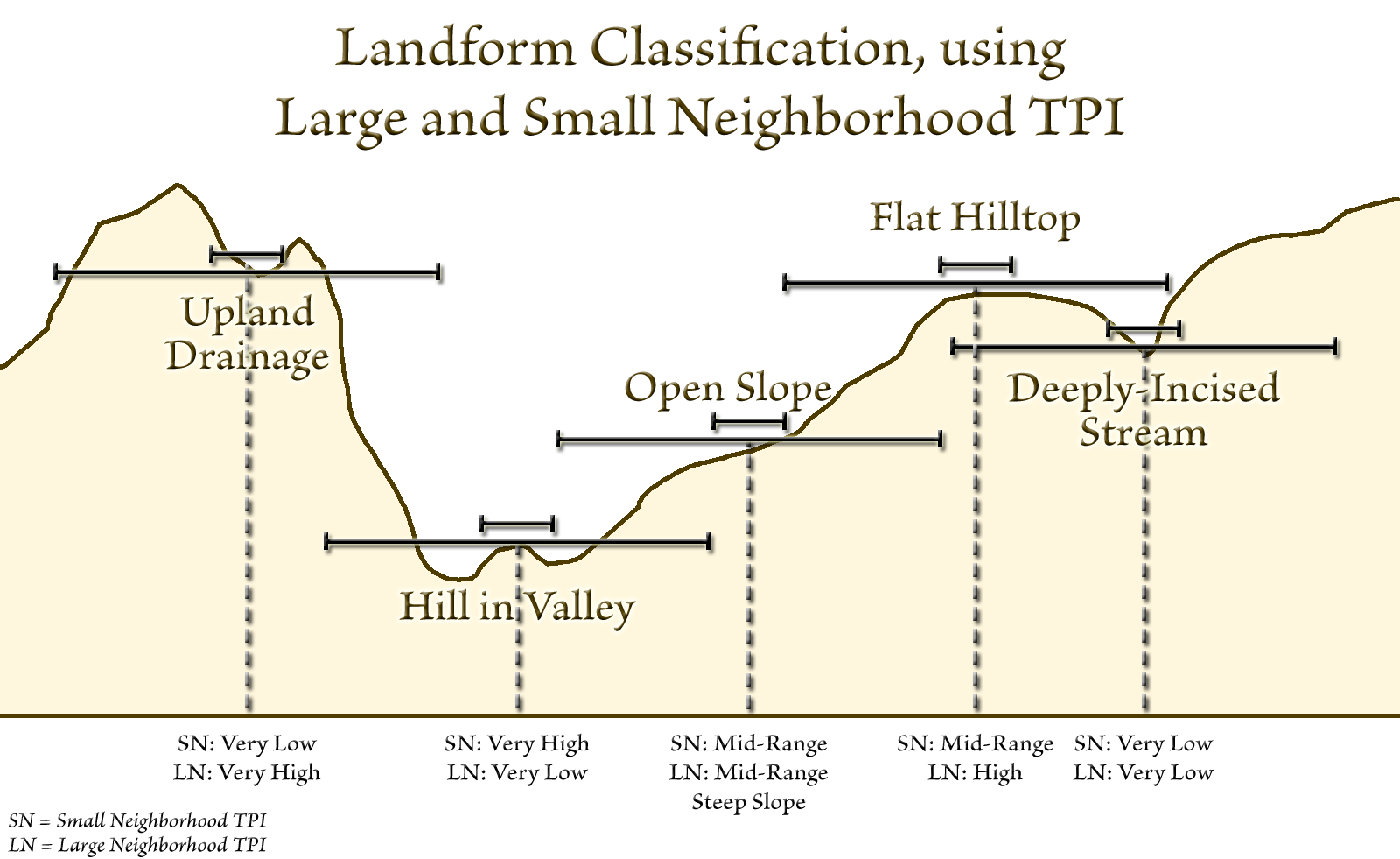
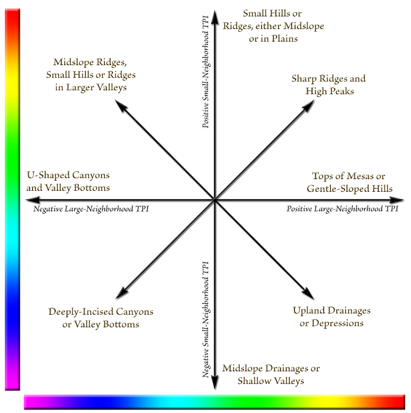
The ten classes, as bundled with the Landform Classification tool, follow the poster with the class names of the extension manual. SN is the small-neighborhood TPI and LN the large-neighborhood TPI, both in standard-deviation units:
| Class | Small-neighborhood TPI | Large-neighborhood TPI | Slope |
|---|---|---|---|
| 1. Canyons, deeply incised streams | SN ≤ −1 | LN ≤ −1 | |
| 2. Midslope drainages, shallow valleys | SN ≤ −1 | −1 < LN < 1 | |
| 3. Upland drainages, headwaters | SN ≤ −1 | LN ≥ 1 | |
| 4. U-shaped valleys | −1 < SN < 1 | LN ≤ −1 | |
| 5. Plains | −1 < SN < 1 | −1 < LN < 1 | ≤ 5° |
| 6. Open slopes | −1 < SN < 1 | −1 < LN < 1 | > 5° |
| 7. Upper slopes, mesas | −1 < SN < 1 | LN ≥ 1 | |
| 8. Local ridges, hills in valleys | SN ≥ 1 | LN ≤ −1 | |
| 9. Midslope ridges, small hills in plains | SN ≥ 1 | −1 < LN < 1 | |
| 10. Mountain tops, high ridges | SN ≥ 1 | LN ≥ 1 |
Slope enters only where both TPIs are near zero, to separate plains from open slopes; everywhere else the two TPIs decide. The ten classes cover every combination of the two indices, so no cell is left unclassified, and since the classes do not overlap the order in which they are tested does not matter.
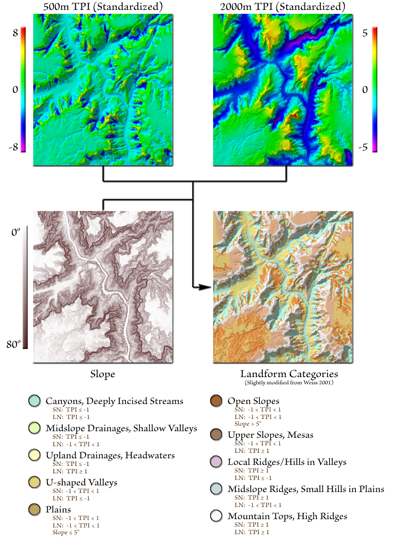
Nothing about the two-scale logic requires standardized units. It is perfectly reasonable to classify landforms from two raw TPI rasters, with both thresholds set in elevation units. Weiss used standard deviations, but they carry the drawback described above: identical shapes can be classified differently depending on the topography around them, so the same 20 m knoll might be a local ridge on a plain and an unremarkable bump in the mountains. Raw thresholds read every knoll of a given height the same way, wherever it is, and for many ecological questions that makes them the more defensible choice. The price is the one Weiss standardized to avoid: raw TPI values span a wider range in a large neighborhood than in a small one, so the two scales need their own thresholds, chosen for the landscape and the question. The Landform Classification tool lets each scale use its own TPI type, and a raw version of the ten-class system is a matter of duplicating the bundled one in the Classification System Builder and entering the thresholds in elevation units.
A worked landscape: the Yazoren Polje
Tağıl and Jenness (2008) applied the whole sequence to a 44 km² karst watershed around the Yazoren Polje in the Marmara region of Turkey, a closed limestone depression drained by a gorge and surrounded by volcanic plateaus. The DEM was a 20 m raster interpolated from 10 m contours, and the analysis area was the watershed plus a 500 m buffer, so that every cell inside the watershed had a full neighborhood. TPI was computed at six circular neighborhoods, 50, 100, 150, 200, 250 and 450 m, and each was classified into four slope-position classes: valley bottom below −1 standard deviation, hilltop above +1, and the rest split at a 6° slope into flat and mid-slope.
Of the six, the 100 m neighborhood did the best job of extracting the features the authors wanted, the terraces along the gorge and the small karst depressions. Those features were too small to be picked out by the larger neighborhoods, and the 50 m neighborhood tended to extract only their edges rather than the features themselves. For landforms, the 50 m and 450 m TPIs were combined with slope, again split at 6°, under Weiss's ten-class criteria. More than half of the area came out as open slopes, which the authors attribute to the several rivers that cut the basin. The polje floor itself was classified as a plain, passing abruptly to open slopes along its northern and southern edges, where the geologic map shows normal faults; and three erosional surfaces at different heights appeared as upper slopes and mesas.
The paper is equally clear about what the classification got wrong. Several closed karst depressions were classified as deeply incised streams and U-shaped valleys, because the rules have no way to distinguish a closed hollow from a valley that drains; their flat floors were plains and their rims open slopes. The terraces showed up as local ridges and midslope ridges, which is what they look like to a two-scale index. Narrow creeks crossing wide flats without forming a broader valley were not identified at all. These are worth remembering as the characteristic behaviors of the method rather than as errors in its application: TPI describes relative height, and landforms that are defined by drainage or by process have to be read from it with care.
Choosing the neighborhood, and the thresholds
There is no single correct neighborhood size or shape, and no single set of thresholds that works everywhere, because there is no single definition of a hill or a valley. The right choices depend on the phenomenon being modeled. A large predator such as a bear or a mountain lion may be aware of the terrain for several hundred meters around it, while a mouse may pay attention to only the nearest 5 to 10 m, so the two call for very different neighborhoods on the same landscape. The same goes for the thresholds: a 10 m rise can be a substantial ridge to a mouse and go unnoticed by a mountain goat, for which 100 m might be the better threshold, and a slope threshold of 5° is usually a judgment rather than a measurement, since there is seldom good information about the slope at which an animal starts to treat the ground as a hillside. An argument for 3° or 10° would be as reasonable unless something specific about the organism or process points to a particular value.
The neighborhood size has little to do with the resolution of the DEM, except at the extremes. The DEM has to be fine enough to describe the terrain inside the neighborhood, so a 10 m neighborhood on a 10 m DEM is meaningless, and a very large neighborhood on a very fine DEM means a great many cells in every neighborhood mean, which costs computing time. Between those limits, the neighborhood is set by the question, not by the data.
For shape, a circle is the most defensible general choice. It extends the same distance in every direction, and for wildlife it is the natural model of an animal's perceptual range: the area around it that it pays attention to. Squares and rectangles reach farther in some directions than others, and an annulus ignores the cells nearest the focal cell. An annulus makes sense when the question is specifically how local conditions compare with more distant ones, but a different shape needs a clear reason behind it.
In practice, the choice is made by trial and error, and nearly everyone who uses the index tries several neighborhoods and thresholds before settling on one. Some strategies make that process quicker and easier to defend:
- Calibrate on features you know. Pick a hill or valley that clearly should be classified a certain way, try combinations of neighborhood size and threshold until that feature comes out right, and then apply the same combination to the rest of the landscape. The TPI Neighborhood Sampler is built for exactly this: it takes a snapshot of the DEM in the map view and, as two sliders move, shows which neighborhood and which threshold classify a chosen feature the way you want, in a window, without writing anything.
- Work on a small piece first. Clip out a small part of the DEM that contains the features of interest. The trial-and-error runs go much faster, and the full DEM is run only once the settings are chosen.
- Try a range of scales and compare. Tağıl and Jenness (2008) computed TPI at six radii and chose the one that extracted their terraces and karst depressions; Guisan et al. (1999) offered four scales to their species models and let the data select among them.
- Consider leaving the index continuous. A classified TPI carries two subjective choices, the neighborhood size and the thresholds; a continuous TPI carries only the first. Classes such as “ridge” are easier for land managers to talk about than “positive index values,” but a continuous TPI is often the more defensible input to a statistical model, because it removes one layer of subjectivity.
- Write down the reasoning. There is no recipe that produces the correct parameters. What a reviewer can fairly ask is that the neighborhood and thresholds were chosen with some thought and logic, and that the logic is defensible for the organism or process being studied.
A classification of hills and valleys with no question behind it is only an academic exercise: it needs to satisfy nobody's idea of a hill but the analyst's, and it is unlikely to be useful for anything else. The index earns its keep when the neighborhood and thresholds are tied to what matters to the organism or process under study.
The six tools at a glance
Four of the tools are geoprocessing tools; the other two are windows, one for authoring the classification systems the others apply and one for trying neighborhoods and thresholds before running them.
| Tool | What it does |
|---|---|
| Topographic Position Index | Computes TPI from a DEM over a circular or annular neighborhood, in any of the five forms above, as floating-point rasters that can be used directly or handed to the classification tools. |
| Slope Position Classification | Classifies one TPI plus slope into slope-position classes using a saved classification system, computing the TPI and slope from the DEM on the fly or taking rasters you already have. Bundled systems: a six-class system adapted from Weiss (2001) in standardized, raw and percentile forms, Dickson and Beier four-class, Corridor Designer four-class, and Land Facet Corridor Designer three-class. |
| Landform Classification | Classifies a small- and a large-neighborhood TPI plus slope into landform classes, again on the fly or from existing rasters. Bundled system: a ten-class system adapted from Weiss (2001). |
| General Raster Classification | Applies a saved system to any single raster, in raw or whole-raster standardized units: the same machinery as the two tools above, without the terrain. |
| Classification System Builder | Creates, edits, duplicates and deletes the classification systems: the classes, their thresholds and units, their names and colors. Systems are saved as JSON files in a per-user folder that survives reinstalling the add-in, and can be shared by copying the files. |
| TPI Neighborhood Sampler | Takes a snapshot of the DEM in the map view and, as two sliders move, paints the TPI for any circular neighborhood and draws any threshold as a line, with a pinned cell's TPI plotted against the radius: a way to find the neighborhood and threshold that classify a known feature the way you want before running the tools. Raw and neighborhood standard deviation scales. |
The tools descend from the Topographic Position Index extension for ArcView 3.x (Jenness 2006), which automated Weiss's methods and introduced saved, shareable criteria sets, and from the TPI tools of the Land Facet Corridor Designer for ArcMap (Jenness, Brost and Beier 2013), which offered the raw index, the neighborhood-standardized form and the whole-raster standardized form, and fixed three-, four- and six-category topographic position tools. The Pro tools replace the fixed category tools with classification systems that carry their own names, colors and units, and compute every neighborhood without Spatial Analyst.
Credits and references
By Jeff Jenness, Jenness Enterprises (www.jennessent.com). The TPI method and the slope-position and landform classifications are the work of Andrew Weiss of The Nature Conservancy; the extension that first automated them was suggested and partly funded by Joyce Miller of the National Oceanic and Atmospheric Administration. The profile and map figures on this page are from the extension manual.
- Beier, P., and B. Brost. 2010. Use of land facets to plan for climate change: conserving the arenas, not the actors. Conservation Biology 24:701–710. doi.org/10.1111/j.1523-1739.2009.01422.x
- Brost, B. M., and P. Beier. 2012. Use of land facets to design linkages for climate change. Ecological Applications 22:87–103. doi.org/10.1890/11-0213.1
- Dickson, B. G., and P. Beier. 2007. Quantifying the influence of topographic position on cougar (Puma concolor) movement in southern California, USA. Journal of Zoology 271:270–277. doi.org/10.1111/j.1469-7998.2006.00215.x
- Guisan, A., S. B. Weiss, and A. D. Weiss. 1999. GLM versus CCA spatial modeling of plant species distribution. Plant Ecology 143:107–122. doi.org/10.1023/A:1009841519580
- Jenness, J. 2006. Topographic Position Index (tpi_jen.avx) extension for ArcView 3.x, v. 1.3a. Jenness Enterprises. jennessent.com/arcview/tpi.htm
- Jenness, J., B. Brost, and P. Beier. 2013. Land Facet Corridor Designer. Available at: corridordesign.org (archived copy at the Internet Archive)
- Jones, K. B., D. T. Heggem, T. G. Wade, A. C. Neale, D. W. Ebert, M. S. Nash, M. H. Mehaffey, K. A. Hermann, A. R. Selle, S. Augustine, I. A. Goodman, J. Pedersen, D. Bolgrien, J. M. Viger, D. Chiang, C. J. Lin, Y. Zhong, J. Baker, and R. D. Van Remortel. 2000. Assessing landscape condition relative to water resources in the western United States: a strategic approach. Environmental Monitoring and Assessment 64:227–245. doi.org/10.1023/A:1006448400047
- Majka, D., J. Jenness, and P. Beier. 2007. CorridorDesigner: ArcGIS tools for designing and evaluating corridors. Available at: corridordesign.org (archived copy at the Internet Archive)
- Tağıl, Ş., and J. Jenness. 2008. GIS-based automated landform classification and topographic, landcover and geologic attributes of landforms around the Yazoren Polje, Turkey. Journal of Applied Sciences 8:910–921. doi.org/10.3923/jas.2008.910.921
- Weiss, A. 2001. Topographic Position and Landforms Analysis. Poster presentation, ESRI User Conference, San Diego, CA. jennessent.com/arcview/TPI_Weiss_poster.htm
- Wilson, J. P., and J. C. Gallant. 2000. Terrain analysis: principles and applications. John Wiley and Sons, New York.
Related tools and pages
- Topographic Position Index
- Slope Position Classification
- Landform Classification
- General Raster Classification
- Classification System Builder
- About Topographic Roughness — the neighborhood measures of how rough the terrain is, and the same lesson about scale.
- About Land Facets — topographic position as the first partition of a landscape into land facets.
- Projecting Rasters — the TPI tools handle geographic DEMs correctly, but if you do project a DEM first, project it with bilinear interpolation.
- TPI Neighborhood Sampler