

Topographic Wetness Index
Summary
Computes the Topographic Wetness Index (TWI, also called the Compound Topographic Index or CTI) for every cell of a DEM: the natural log of the specific catchment area divided by the local slope gradient (Beven and Kirkby 1979). The index combines the two things about the shape of the land that decide where water collects: how much ground drains to a cell, and how steep the cell is, and consequently how quickly water drains off it. High values mark cells with a large upslope area and a gentle slope, the valley bottoms, hollows and flats where water arrives and lingers; low values mark ridges and steep, diverging slopes that shed it. It is a purely topographic estimate of relative wetness, built from the shape of the land alone, with no knowledge of rainfall, soils or subsurface flow. The sink filling, flow direction and flow accumulation it needs are computed internally, with a choice of D8, MFD or D-Infinity flow direction methods, so no Spatial Analyst extension is required; you may instead supply a filled DEM and a flow-accumulation raster of your own, and you may save the ones the tool computes.
The idea
Beven and Kirkby (1979) proposed the index as part of TOPMODEL, a rainfall-runoff model they describe as “a model for humid temperate areas.” The question it answers is simple: where on a landscape does water tend to collect? Two things decide that. Water arrives at a place in proportion to how much ground drains to it, and it leaves in proportion to how steep the place is. A cell at the bottom of a broad basin receives water from every cell above it and, being nearly level, passes it on slowly. A cell on a ridge crest receives nothing from anywhere and sheds what falls on it at once. The wetness index puts the two together as a ratio and takes its logarithm:
Here a is the specific catchment area, explained in the next section, and tan β is the slope gradient at the cell, its rise over run. That is the tangent of the slope angle β, which is percent slope divided by 100, and not the slope in degrees or in percent. The logarithm is there because the ratio spans an enormous range, from values near 0 on a steep ridge to millions or more at the mouth of a large basin; the log compresses that into a scale of roughly 0 to 25 that can be mapped and compared. The index rises as catchment area grows, because larger areas collect more water in general, and rises as slope falls, because water moves more slowly across gentle ground. The lecture calls it a sort of measure of water pressure or concentration at a location, and that is a fair way to picture it.
The same quantity goes by several names. Beven and Kirkby wrote it as ln(a/tan β) and called it a topographic index; the USGS distributed it with the HYDRO1k global elevation derivatives as the Compound Topographic Index, “commonly referred to as the Wetness Index,” following Moore et al. (1991); Topographic Wetness Index is the name most ecological papers use now, and the name this tool uses.
Specific catchment area and the unit contour length
Catchment area is easy: it is the area of ground that drains to a point, the watershed above it. Specific catchment area is the part that confuses people, and it took me years to get a handle on it, because watersheds do not always drain to a point. Picture a spring pouring water over a convex surface such as a cone. As the water runs down, it spreads out. There is no single point where the flow from the spring collects; the outlet of that little watershed is a line along the cone, and the watershed that feeds the line is a fan-shaped strip between two flow paths.
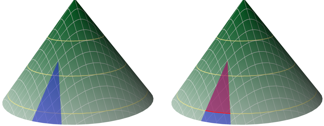
That is what specific catchment area does. It is the catchment area divided by the length of the line across which the water leaves it, the length of the contour segment through which the flow passes. The literature calls that line the unit contour length (Beven and Kirkby 1979; Sørensen et al. 2006) and defines the specific catchment area as the upstream area per unit width of contour (Moore et al. 1991; Yang et al. 2011). Its units are square meters divided by meters, which reduces mathematically to meters, but the units make better sense left as they are: read them as square meters of watershed per meter of outlet line. On a diverging surface like the cone, the area per meter of outlet is small; where flow converges into a channel, all of the watershed passes through a short outlet line and the number is large. That is why the index needs the specific area and not the plain one: a point on the cone has a catchment area of essentially zero, and the index would have nothing to work with.
What a raster does with this
Raster flow analysis changes the picture in one important way. Flow direction and flow accumulation treat every cell as a watershed outlet in its own right, and the accumulation raster tells you how many cells drain into each cell. You cannot set the whole red line on the cone as an outlet; each cell along it gets its own count. So in a raster the outlet line of a cell's watershed is the edge of that cell, the unit contour length is the cell size, and the derivation runs in three lines:
| Quantity | Formula | Units |
|---|---|---|
| Catchment area of a cell | (flow accumulation + 1) × cell size × cell size | m² |
| Unit contour length | cell size | m |
| Specific catchment area, a | (flow accumulation + 1) × cell size | m² per m |
One cell size cancels. The “+ 1” is there because Esri's Flow Accumulation, and this tool's own accumulation, count the cells upstream of a cell and not the cell itself. This means that the Flow Accumulation algorithms do not consider the cell itself to be contributing to its own accumulated flow, so we add “1” to the flow accumulation value in order to force the cell's catchment area to include the cell itself. Rain that falls on a cell is in that cell. Adding one also keeps the logarithm defined at the head of every drainage, where the count is zero and ln(0) would otherwise be the result. This tool computes the specific catchment area exactly as the table shows.
A note on Geographic DEMs: On a geographic (latitude/longitude) DEM a cell is not square on the ground: at 36° north a one-arc-second cell is about 25 m east to west and 31 m north to south, and the east-west span changes with every row. The tool measures both spans in meters on the spheroid for each row, takes their product as the cell area, and takes the square root of that area, the side of a square of the same size, as the unit contour length, about 28 m in this example. One length serves every cell whatever direction its water leaves by, for the same reason the diagonal is not used for diagonal flow: a divisor that changed with the direction of flow would tilt the index by compass direction for no physical reason.
One more raster question is which edge of the cell to divide by. Water leaves a cell in one of eight directions under the D8 rule, and when it leaves diagonally the line it crosses is, strictly, the cell's diagonal, 1.414 times the edge. Dividing by the diagonal for diagonal flow and the edge for the rest would make the index systematically higher wherever water happens to flow north, east, south or west, and nothing in the real world justifies that, so this tool divides every cell by the same constant, the cell size, whatever direction the water takes.
A worked example
The table shows the index for a 30 m DEM at a few combinations of flow accumulation and slope. Flow accumulation is Esri's count of upslope cells, so the first row is a cell at the head of a drainage with nothing above it and the last is a cell with 10,000 cells, nine square kilometers, draining through it. The constant added to the slope is the tool's default of 0.001, which matters only in the level column.
| Upslope cells | Catchment area (m²) | Specific catchment area a (m²/m) | TWI, level ground | TWI, 5° (tan 0.087) | TWI, 20° (tan 0.364) | TWI, 45° (tan 1.0) |
|---|---|---|---|---|---|---|
| 0 | 900 | 30 | 10.3 | 5.8 | 4.4 | 3.4 |
| 9 | 9,000 | 300 | 12.6 | 8.1 | 6.7 | 5.7 |
| 99 | 90,000 | 3,000 | 14.9 | 10.4 | 9.0 | 8.0 |
| 999 | 900,000 | 30,000 | 17.2 | 12.7 | 11.3 | 10.3 |
| 9,999 | 9,000,000 | 300,000 | 19.5 | 15.0 | 13.6 | 12.6 |
Read down a column and each tenfold increase in catchment adds 2.3 to the index, which is ln(10): the log turns multiplication into addition. Read across a row and steepness pulls the index down, but more gently, because going from 5° to 45° multiplies the tangent by only 11.4, worth 2.4 on the log scale. Now look at the level column. A single cell with nothing draining into it scores 10.3 on level ground, about the same as a hundred-cell watershed at 5°. That is the added constant talking: on a perfectly level cell the tangent is zero, the ratio would be infinite, and the small constant added to the slope is what keeps it finite, but it keeps it very large. A lake surface, a playa, a flat roof of a mesa, or a level stretch of DEM produced by an integer elevation grid will all score near the top of the map. Whether that is right depends on what you are asking; a flat is a place where water lingers, but a flat on a summit is not wet. The slope section says more about that constant.
The slope term
The slope is computed from the original DEM, not from the filled one. The DEM is filled only so that flow routing does not get stuck in sinks; for every other purpose the true, unmodified surface is the one to use, and a filled DEM would report zero slope across the floor of every filled depression. The gradient is Horn's method, the same 3 × 3 operator as Esri's Slope tool, and its output is a rise over run, the tangent of the slope angle. Because it is a tangent, the DEM's elevation units must match its horizontal units: the tool reads the units from the DEM's vertical coordinate system when it has one and asks you only when the DEM does not say, and it converts internally so that a DEM in feet gives the same gradient as the same terrain in meters.
On a projected DEM the slope is Planar by default, measured in the projection's own plane with the raster's cell size, which matches Esri's Slope tool with the Planar method and is the right choice for nearly every projected DEM. The Geodesic choice measures the distances between cell centers on the spheroid instead, correcting for the projection's scale distortion; on a UTM or State Plane DEM it is essentially identical to Planar, and it earns its place only on large-extent or highly distorted projections such as Web Mercator across a wide range of latitudes. It is a true-ground-distance correction and does not attempt to reproduce Esri's geocentric Geodesic method. On a geographic DEM the choice is disabled: slope is always computed per row on the spheroid, because a degree of longitude is a different distance at every latitude.
The value added to slope is a small constant added to the gradient before dividing, so that a level cell does not divide by zero. The default 0.001 is the value the USGS used for flat cells in the HYDRO1k wetness index, and the value my Watershed lab uses; the tool adds it to every cell's slope, level or not. Its effect is confined to nearly level ground: at 5° the tangent is 0.0875, the constant changes the index by 0.01, and at any real slope it does nothing you could see. On a perfectly level cell it is the whole denominator. The HYDRO1k documentation substitutes 0.001 for the slope of a flat cell rather than adding it everywhere. The two conventions give the same value on flat cells, and elsewhere they differ by ln((tan β + 0.001) / tan β): about a hundredth at 5°, 0.06 at 1°, 0.11 at 0.5°, and 0.21 on the gentlest slope a 30 m DEM with whole-meter elevations can express, a rise of 1 m across the 240 m span of Horn's window. On ground that steep or steeper the difference is invisible; on nearly level ground it is a few tenths. If the level areas of your DEM are scoring higher than you believe they should, raising the constant to 0.01 lowers a level cell's index by 2.3 and moves a 5° cell by only 0.1. When the flats are lakes, mask the lakes out of the output rather than out of the DEM: a NoData hole in the DEM is an outlet, as the next section explains, and every cell downstream of a masked lake would lose the lake's catchment.
How the hydrology is computed
Everything is done inside the tool with NumPy, so it runs at any ArcGIS Pro license and needs no Spatial Analyst extension. Three steps produce the flow accumulation.
Fill. Real DEMs are full of small closed depressions, some real and most of them artifacts, and water routed across such a surface stops in every one of them. Sinks are removed with the priority-flood algorithm of Barnes, Lehman and Mulla (2014), which floods the surface inward from its edges, raising each depression to the level of its spill point. The result matches Esri's Fill tool cell for cell.
Flow direction. Each cell of the filled surface passes its water to one or more of its eight neighbors, by the routing method you choose; the next section describes the three. Cells on a flat, which have no downhill neighbor, drain across the flat to its nearest exit, so every cell drains somewhere and no water circles forever.
Flow accumulation. Following the directions downstream, each cell's value is the area whose water passes through it, in cells, not counting itself, which is the convention of Esri's Flow Accumulation tool. Under D8 that is a whole number of cells; under the two dispersive methods (Multiple Flow Direction [MFD] and D-∞ [D-Infinity or DINF]), it is fractional, because upstream cells send only shares of their area. If you need a result that reproduces an Esri workflow exactly, run Esri's Fill, Flow Direction and Flow Accumulation, supply the accumulation raster in the optional group of the dialog, and the tool will use it directly and skip its own hydrology; it still needs the original DEM for the slope.
Three ways to route the water: D8, D-Infinity and MFD
These are the same three algorithms that Esri's Flow Direction and Flow Accumulation tools offer, but not Esri's implementations of them. This tool is designed to run without Spatial Analyst, so it carries its own versions of all three, written from the published descriptions. How closely their results match Esri's is reported below.
D8 (O'Callaghan and Mark 1984), the default, sends all of a cell's water to the one neighbor that lies most steeply below it. That is the right thing in a channel and the wrong thing on the cone of the lecture, where water genuinely diverges: under D8 a cell on a convex hillside receives water only from the one thread of cells that happens to point at it, and its catchment stays small no matter how much ground lies above it. As the lecture puts it, calculating specific catchment area is difficult on a convex surface, and fortunately we are usually more interested in the index in concave regions, where flow converges and D8 does well. D8 is also Esri's default method for calculating flow accumulation, and the simplest method to understand.
D-Infinity (Tarboton 1997) fits eight triangular facets around the cell, one between each pair of adjacent neighbors, and takes the steepest facet's downslope direction as a continuous angle rather than one of eight compass points. The cell's water is then split between the two neighbors that bracket that angle, in proportion to how close the angle is to each: a direction 30° from the east neighbor and 15° from the northeast one sends two thirds northeast and one third east. Each receiving cell does the same in its turn, so on the cone the water from a point spreads into a widening fan, which is the purple strip of the lecture slide, and in a channel the two shares collapse toward a single thread.
The steepest facet direction is essentially the cell's aspect, the direction the ground faces, computed on the facets rather than on Horn's 3 × 3 window. Tarboton reports it in the mathematical convention, as a polar angle with zero at east and increasing counter-clockwise, rather than as a compass bearing with zero at north and increasing clockwise, so the angle in a D-Infinity flow-direction raster does not read like an aspect raster even though it points the same way. The aspect tools accept such a raster through their Input aspect convention setting, described on the Aspect Zonal Statistics as Table page.
MFD, the multiple-flow-direction method of Quinn et al. (1991), sends a share to every lower neighbor, weighted by the slope toward it and by the contour length that neighbor represents: half a cell width for a cardinal neighbor and 0.354 of a cell width for a diagonal one, from the geometric construction in their Figure 1, which this tool uses. The tool uses the adaptive form of Qin et al. (2007), which is also what Esri's MFD option implements: the slope is raised to an exponent that grows with the local steepness, so that flow spreads widely on gentle ground and concentrates on steep ground. MFD disperses more than D-Infinity, and on a plane it spreads water sideways where none should go; Tarboton's tests on cones and planes found D-Infinity closer to the true contributing area, while Sørensen et al. (2006), who tested many routing choices against measured groundwater levels, soil moisture, soil pH and plant species richness at two boreal forest sites, found that no single method was best for every variable.
How do our outputs compare with Esri's? On a projected floating-point DEM of the Grand Canyon, the tool's D8 accumulation agrees with Esri's Flow Accumulation on 99.9 percent of cells and its D-Infinity on 99.8 percent, the remainder being flats, where the exit a flat drains to is a matter of convention. Integer DEMs are harder to match, because two or three neighbors often tie for steepest and something has to break the tie; this tool breaks it in the same order Esri's Flow Direction does, and on a 30 m integer DEM its D8 accumulation matched Esri's exactly on 85 percent of cells and within 5 percent on 91 percent, with the rest again on flats. Its MFD agrees with Esri's within 5 percent on 83 percent of cells, with a correlation of 0.97 between the two on the log scale; Esri does not publish every detail of its MFD implementation, so the two are close rather than identical. If you need an Esri result exactly, then just calculate that Flow Accumulation manually using Esri's Flow Accumulation tool, then give that raster to this TWI tool, as described above.
Whichever method routes the water, the specific catchment area is the same formula: the accumulation plus one, times the cell size. It is tempting to think that a cell sending water to two neighbors should be divided by two cell widths, but the divisor is the width of the cell whose value is being computed, not the number of cells it sends water to; Tarboton (1997) defines the specific catchment area as A/L with L the pixel width for every routing method, and his cone test uses it. The spreading is already expressed in the smaller shares each downslope cell receives. Divide again by the number of receivers and the values on a cone come out about half of the truth. Quinn et al. (1991) did set it up differently in their own paper: they divided the upslope area by the sum of the contour lengths of all the downhill directions, and used a weighted mean of the downhill gradients as the slope, so their divisor grows with the number of directions a cell drains in. This tool follows Tarboton's convention instead, which is also what Esri's Flow Accumulation delivers, so that one specific-catchment-area formula serves all three methods. The table shows the tool's D8 and D-Infinity results on a cone with unit cells, where the true specific catchment area on the ring at radius r is r/2 for every cell of the ring:
| Ring radius | True value r/2 | D8: min, median, max | D-Infinity: min, median, max |
|---|---|---|---|
| 10 | 5 | 1, 5.0, 10 | 3.8, 4.9, 6.8 |
| 20 | 10 | 1, 8.5, 20 | 7.3, 9.2, 12.9 |
| 40 | 20 | 1, 18, 40 | 14.1, 17.9, 25.1 |
| 60 | 30 | 1, 25, 60 | 21.0, 26.7, 37.3 |
D8 shows the thread problem. Around any ring its values scatter from 1, on the cells the threads bypass, up to double the truth on the eight cells where the cardinal and diagonal rays run; the median sits near the true value, but no single cell can be trusted. D-Infinity, divided by one cell width, stays near the true value all the way around.
The raster's edge and every NoData cell act as outlets. The fill starts from the cells that touch NoData or the edge, and a flat beside NoData drains into it, so water that reaches either one leaves the analysis. Two consequences follow. A DEM clipped across a drainage loses the catchment of every stream that enters from outside the clip, and the wetness index along those streams comes out too low; use a DEM that covers the full upstream watershed of the area of interest, and clip the output instead. And a lake or any other area set to NoData inside the DEM swallows the water that flows into it, cutting off every cell downstream, which is why the section above recommends masking lakes out of the output, not the DEM.
Reading the map
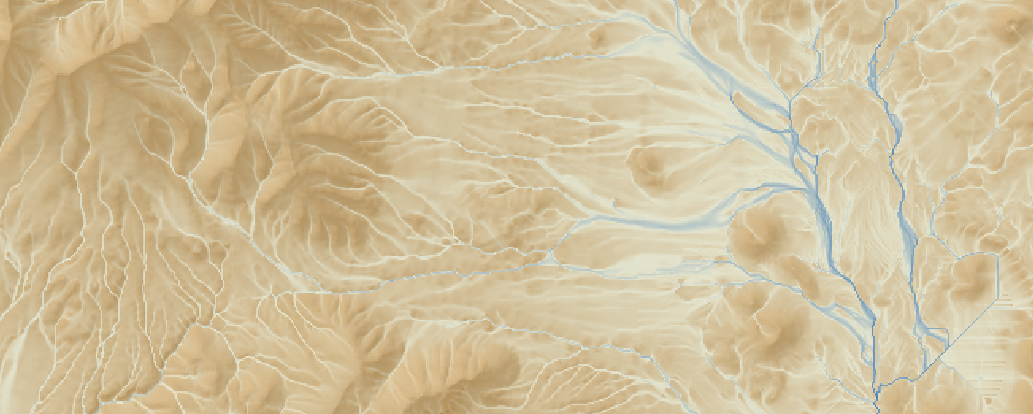
The output is drawn with a tan-to-blue ramp, dry to wet. The high, blue values trace the drainage network and pool in every basin, meadow and flat; the low, tan values sit on the ridges, the noses of spurs and the steep faces. In the Flagstaff DEM the Watershed lab works on, the high values occur in both the meadows and the drainage bottoms, which is what the index was built to find: the places on a landscape where water arrives and stays. If those features matter to a species you manage, this raster is a cheap and repeatable way to map them from elevation alone. The lecture suggests two other uses: finding locations vulnerable to flooding, and finding places where water may collect, tinajas and natural catchments in the desert.
Keep in mind what the index leaves out. It is built entirely from the surface topography, so it probably describes actual soil wetness best in mesic areas that receive steady rain, where the water the terrain would collect is actually there to be collected. Beven and Kirkby framed the model it comes from as one for humid temperate areas. The index pays no attention to aquifers or subsurface structure, and it is normal for xeric or desert areas to have enormously large drainages, be flat as a table, and still be dry as a bone: even substantial rainfall upstream can drain entirely into the ground before it reaches some downstream areas, and those areas will score near the top of the map regardless. In the desert Southwest the water that matters ecologically is more often associated with springs and exposed aquifers than with the wetness index, and a spring on a hillside will never show up in it. Use the index as a map of where the terrain would put water, and let soils and hydrology say whether the water is there.
Comparing wetness indices from different sources
Published TWI values are not comparable across studies unless the recipes match, and the recipes rarely do. The table lists the constant offsets that different formulas introduce; each shifts every cell by the same amount, so the maps look the same and the rankings agree, but the numbers differ.
| Recipe difference | Effect on every cell | Size, for a 30 m DEM |
|---|---|---|
| Catchment area used in place of specific catchment area (flow accumulation multiplied by the cell area instead of the cell size) | adds ln(cell size) | +3.4 |
| Percent slope used in place of the gradient (tan β) | subtracts ln(100) | −4.6 |
| Both of the above together | adds ln(cell size) − ln(100) | −1.2 |
| Distances in kilometers instead of meters | subtracts ln(1000) | −6.9 |
Two other differences are not constant offsets and change the pattern itself. The flow-routing method, D8 against MFD or D-Infinity, redistributes the upslope area on every hillside, as the hydrology section describes. And the DEM's resolution changes the catchment counts: Yang et al. (2011) show that the upslope contributing area at a given location grows as the DEM becomes coarser, most strongly in upslope positions and least near the bottoms of drainages, so a wetness index from a 10 m DEM and one from a 90 m DEM are different surfaces, not the same surface at two levels of detail. Within one study, use one DEM, one routing method and one formula, and compare values only with each other.
A tour of the dialog
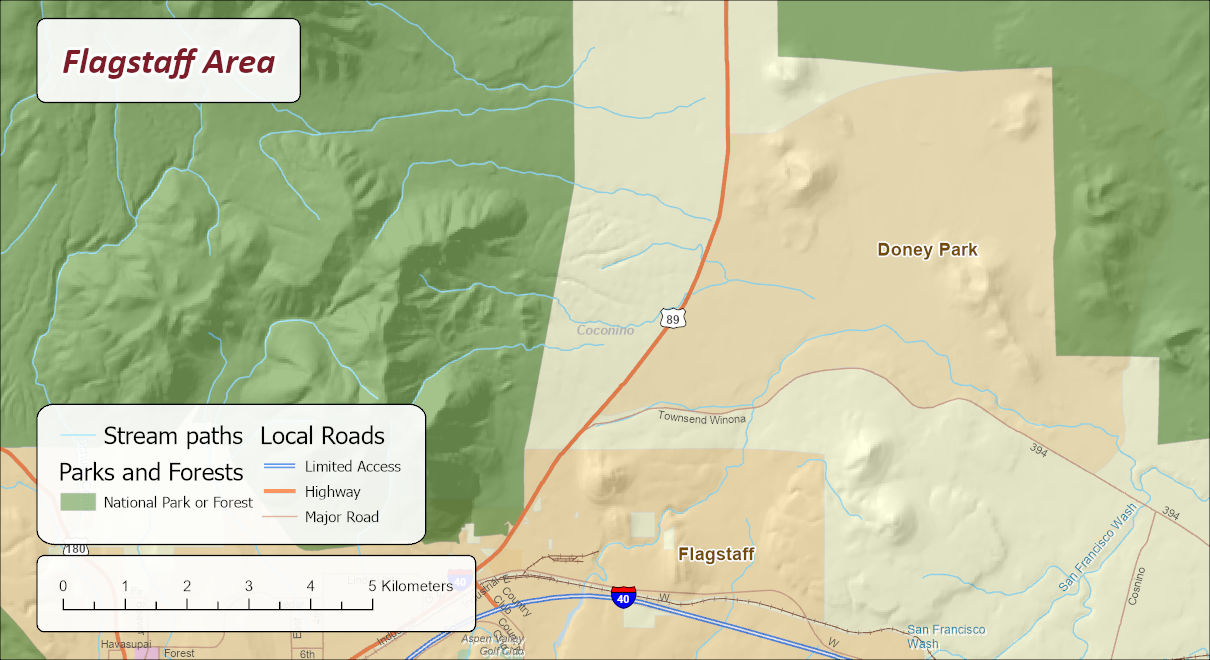
The examples use a DEM of the country just north of Flagstaff, Arizona, with 28.08 m cells in NAD 1983 UTM Zone 12N: the eastern flank of the San Francisco Peaks on the left, US 89 running north through the middle, the cinder cones and the broad, gently sloping plain of Doney Park on the right, and the washes that gather it all toward the San Francisco Wash in the southeast corner. It is the Schultz Pass and Doney Park country of the figure above.
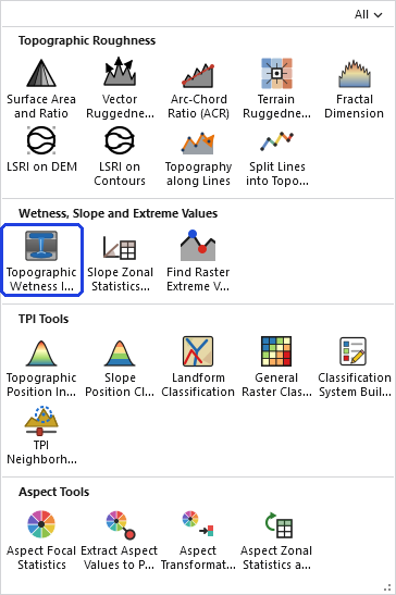
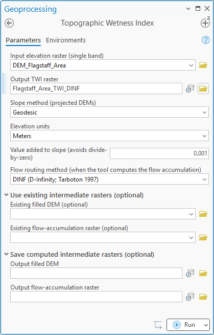
The dialog asks for the DEM, an output name, the slope method for projected DEMs, the value added to slope, and the flow routing method, which is greyed out when you supply an accumulation raster of your own. An Elevation units row is filled in and locked when the DEM carries a vertical coordinate system; when it does not, the row is editable and shows the units from the last run, so check it. The slope method, the constant and the routing method are also remembered from the last run. Below those sit two collapsed groups. Use existing intermediate rasters takes a filled DEM, a flow-accumulation raster, or both; either must share the input DEM's grid exactly, the same extent, cell size and alignment, and supplying the accumulation raster makes the filled DEM unnecessary. Save computed intermediate rasters writes the filled DEM and the flow accumulation the tool computes, for reuse or inspection. Each save option is offered only when the tool actually computes that raster; supply a flow-accumulation raster and both save rows are disabled, because there is nothing of the tool's own to save.
The same ground under the three flow direction methods
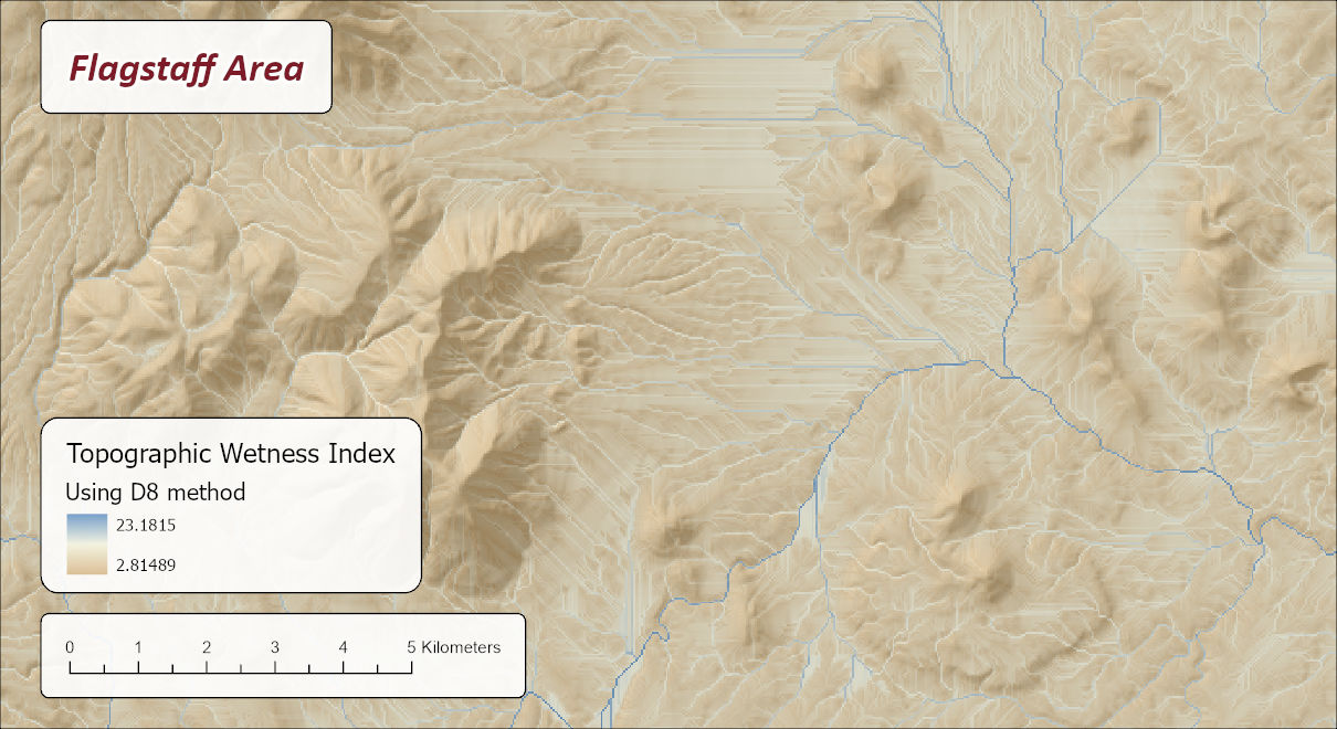
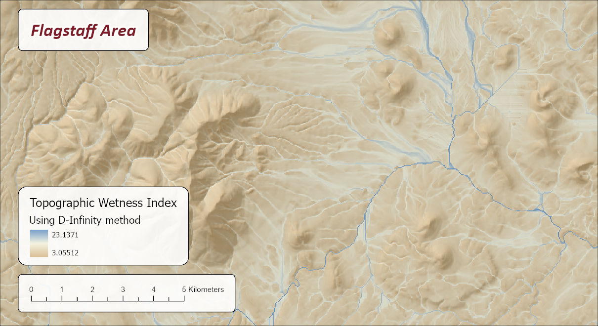
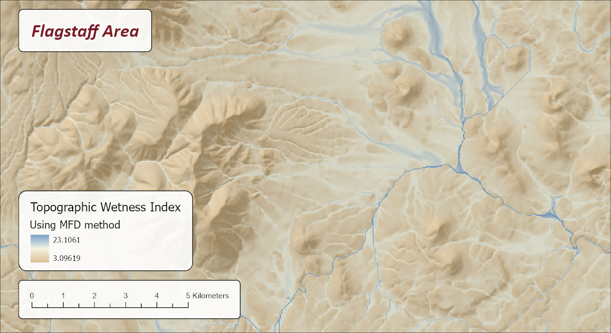
Look first at the plain east of the Peaks, the pale ground between the forest and Doney Park. Under D8 it is covered with closely spaced parallel streaks. That is the thread problem of the cone on a real landscape: every cell sends all of its water to one neighbor, so on a smooth slope the flow lines never merge and never spread, and the index draws each one as a separate hairline of wetness with dry ground between. Under D-Infinity and MFD the same ground grades naturally from the drier hillsides down into the washes, with wetter aprons below the slopes and broad fans where the washes open out onto the plain, which is how water actually behaves on ground like this. D8 is much more constrained into narrow channels; the two dispersive methods spread the contributing area sideways across the slope, and the difference is what the eye picks up first. The main washes, where flow converges, look nearly the same in all three, and the maxima agree to within a tenth, 23.18, 23.14 and 23.11, because the total area draining through a channel does not depend on how the hillsides delivered it. The minima rise a little from D8 to the dispersive methods, 2.81 to 3.06 and 3.10, because under MFD and D-Infinity even a ridge cell receives some share from its neighbors, so no cell is left with only its own area.
The tool reports its progress through the fill, the flow direction, the accumulation and the slope. The messages record the formula and the constant added to the slope, and the output raster's metadata carries the same provenance. The output is a floating-point raster with statistics and a histogram already computed, NoData wherever the DEM is NoData, and the dry-to-wet ramp applied by default. Outputs may go into a geodatabase or a folder; in a folder, a name without an extension becomes a GeoTIFF.
The tool holds the whole DEM in memory at once, so the memory it needs grows with the number of cells. On most DEMs that is no concern. On a very large one the tool may need more memory than your computer has free, and then one of two things happens: Windows starts using the disk as overflow memory and the tool slows to a crawl, or the tool stops with an out-of-memory error. There is no fixed limit; it depends on how much memory your computer has free. If a DEM is too large, clip it to the area you need first.
ModelBuilder
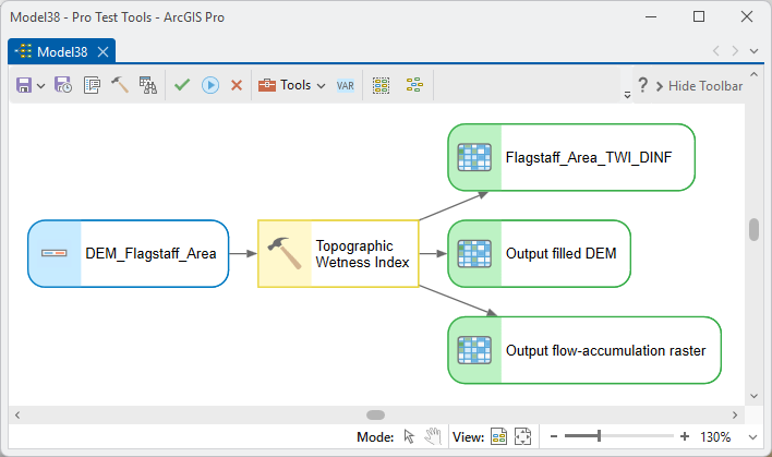
Parameters
| Label | Explanation | Data type |
|---|---|---|
| Input elevation raster (single band)Required · in_raster | The DEM. Must be single band; projected or geographic. Unless you supply a flow-accumulation raster below, this DEM is filled and flow-routed internally. The slope term always comes from this original, unfilled DEM. | Raster Layer |
| Output TWI rasterRequired · out_raster | The wetness index, ln(a / (tan β + the added constant)), as a floating-point raster. Higher is wetter. NoData outside the valid DEM area. A name is suggested from the input and a dry-to-wet color ramp is applied. | Raster Dataset |
| Slope method (projected DEMs)Optional · slope_method | Planar (the default) measures slope in the projection's plane with the raster's cell size, matching Esri's Slope tool; Geodesic uses true ground distances on the spheroid. Disabled for geographic DEMs, which are always computed per row on the spheroid. | String |
| Elevation unitsOptional · elev_units | Meters or Feet. Filled in and locked from the DEM's vertical coordinate system when it has one; you are asked only when the DEM does not say. Keeps the gradient dimensionless whatever units the DEM uses. | String |
| Value added to slope (avoids divide-by-zero)Required · slope_epsilon | A small positive constant added to every cell's slope gradient before dividing. Default 0.001, the HYDRO1k value. Larger values pull level cells toward lower TWI; smaller values push them higher; sloping cells are unaffected. | Double |
| Flow routing method (when the tool computes the flow accumulation)Optional · flow_method | D8 (single flow direction), the default; MFD (multiple flow direction; Qin et al. 2007); or DINF (D-Infinity; Tarboton 1997), as described above. Disabled when you supply your own flow-accumulation raster, because the routing is then already done. | String |
| Existing filled DEM (optional)Optional · in_filled_dem | A depression-filled version of the input DEM to route flow on, so the tool skips its own fill. Must share the input DEM's grid. Ignored if a flow-accumulation raster is also supplied. In the group Use existing intermediate rasters. | Raster Layer |
| Existing flow-accumulation raster (optional)Optional · in_flow_accumulation | A pre-computed flow accumulation, upstream cell count, from Esri's Flow Accumulation (any flow-direction type) or from this tool. The tool then skips filling, flow direction and accumulation and uses it directly. Must share the input DEM's grid. Same group. | Raster Layer |
| Output filled DEMOptional · out_filled_dem | Saves the filled DEM the tool computes. Available only when the tool computes the fill. In the group Save computed intermediate rasters. | Raster Dataset |
| Output flow-accumulation rasterOptional · out_flow_accumulation | Saves the flow accumulation the tool computes, upslope area in cells excluding the cell itself, fractional under MFD and D-Infinity. Available only when the tool computes the accumulation. Same group. | Raster Dataset |
Python
import arcpy
arcpy.ImportToolbox(r"C:\path\to\JennessEnterprisesTools.pyt")  # your install path
# TWI from a DEM, letting the tool fill and flow-route internally,
# and keeping the flow accumulation it computes.
arcpy.jenness.TopographicWetnessIndex(
    in_raster=r"C:\Project\Elev.gdb\DEM",
    out_raster=r"C:\Project\Elev.gdb\DEM_TWI",
    slope_method="Planar", elev_units="Meters", slope_epsilon=0.001,
    flow_method="D8 (single flow direction)",
    out_flow_accumulation=r"C:\Project\Elev.gdb\DEM_FlowAcc")
# The same with D-Infinity routing. The other string is
# "MFD (multiple flow direction; Qin et al. 2007)".
arcpy.jenness.TopographicWetnessIndex(
    in_raster=r"C:\Project\Elev.gdb\DEM",
    out_raster=r"C:\Project\Elev.gdb\DEM_TWI_Dinf",
    slope_method="Planar", elev_units="Meters", slope_epsilon=0.001,
    flow_method="DINF (D-Infinity; Tarboton 1997)")
# TWI on an Esri flow accumulation (for example one computed with MFD).
arcpy.jenness.TopographicWetnessIndex(
    in_raster=r"C:\Project\Elev.gdb\DEM",
    out_raster=r"C:\Project\Elev.gdb\DEM_TWI_MFD",
    slope_method="Planar", elev_units="Meters", slope_epsilon=0.001,
    in_flow_accumulation=r"C:\Project\Elev.gdb\DEM_FlowAcc_MFD")
Recommended citation
Credits and references
By Jeff Jenness, Jenness Enterprises (www.jennessent.com). The index is Beven and Kirkby's; the sink filling is the priority-flood algorithm of Barnes, Lehman and Mulla; the flow routing follows O'Callaghan and Mark (D8), Tarboton (D-Infinity) and Quinn et al. with the exponent of Qin et al. (MFD). The explanation of specific catchment area follows my Topographic Roughness lecture and the Watershed lab exercises of my GIS course.
- Barnes, R., C. Lehman, and D. Mulla. 2014. Priority-flood: an optimal depression-filling and watershed-labeling algorithm for digital elevation models. Computers & Geosciences 62:117–127. doi.org/10.1016/j.cageo.2013.04.024
- Beven, K. J., and M. J. Kirkby. 1979. A physically based, variable contributing area model of basin hydrology. Hydrological Sciences Bulletin 24:43–69. doi.org/10.1080/02626667909491834
- Jenness, J. Topographic roughness. Lecture, GIS for wildlife and forestry courses, Jenness Enterprises. Slides. Accessed on 28 September 2026.
- Moore, I. D., R. B. Grayson, and A. R. Ladson. 1991. Digital terrain modelling: a review of hydrological, geomorphological, and biological applications. Hydrological Processes 5:3–30. doi.org/10.1002/hyp.3360050103
- O'Callaghan, J. F., and D. M. Mark. 1984. The extraction of drainage networks from digital elevation data. Computer Vision, Graphics, and Image Processing 28:323–344. doi.org/10.1016/S0734-189X(84)80011-0
- Qin, C., A.-X. Zhu, T. Pei, B. Li, C. Zhou, and L. Yang. 2007. An adaptive approach to selecting a flow-partition exponent for a multiple-flow-direction algorithm. International Journal of Geographical Information Science 21:443–458. doi.org/10.1080/13658810601073240
- Quinn, P., K. Beven, P. Chevallier, and O. Planchon. 1991. The prediction of hillslope flow paths for distributed hydrological modelling using digital terrain models. Hydrological Processes 5:59–79. doi.org/10.1002/hyp.3360050106
- Sørensen, R., U. Zinko, and J. Seibert. 2006. On the calculation of the topographic wetness index: evaluation of different methods based on field observations. Hydrology and Earth System Sciences 10:101–112. doi.org/10.5194/hess-10-101-2006
- Tarboton, D. G. 1997. A new method for the determination of flow directions and upslope areas in grid digital elevation models. Water Resources Research 33:309–319. doi.org/10.1029/96WR03137
- U.S. Geological Survey, EROS Data Center. HYDRO1k elevation derivative database: documentation (section 3.2.5, Compound Topographic Index). usgs.gov/centers/eros/science/usgs-eros-archive-digital-elevation-hydro1k. Accessed on 28 September 2026.
- Yang, X., G. Tang, C. Xiao, Y. Gao, and S. Zhu. 2011. The scaling method of specific catchment area from DEMs. Journal of Geographical Sciences 21:689–704. doi.org/10.1007/s11442-011-0873-2
Licensing information
Works at every ArcGIS Pro license level (Basic, Standard, Advanced). No extension licenses are required; the sink filling, flow direction, flow accumulation and slope are all computed internally, without Spatial Analyst.
Related tools and pages
- Projecting Rasters — why a nearest-neighbor DEM corrupts modeled flow, and this index with it.
- Find Raster Extreme Values — the peaks and sinks of a DEM as points, each with its prominence or depth.
- Slope Zonal Statistics as Table — slope summarized by zone, in angle space.
- Slope Position Classification — valley bottoms and ridges classified from position rather than from flow.
- About Topographic Roughness — where the wetness index sits among the toolbox's terrain measures.