

Vector Ruggedness Measure (VRM)
Summary
Computes the Vector Ruggedness Measure of Sappington, Longshore and Thompson (2007): a roughness index that measures how much the directions the terrain faces vary within a neighborhood of each cell, independent of how steep that neighborhood is on average. Every cell has a unit vector pointing straight out of its surface; on a smooth slope the vectors of neighboring cells all point the same way, and on broken terrain they scatter. VRM is the three-dimensional version of the circular variance used for compass directions (Fisher 1993), and it runs from 0 for a flat or uniformly sloped neighborhood to 1 for maximum dispersion. The neighborhood is a circle of any radius, in cells or ground units; the tool is correct on geographic (latitude/longitude) DEMs; and the local detrending of Dilts et al. (2023) is available as an option for the VRM-L variant. No Spatial Analyst license is needed.
Why a ruggedness measure that ignores slope
Most ruggedness indices are built from elevation differences, and so they are strongly correlated with slope: a smooth, steep hillside has elevations that genuinely differ from one side to the other, and it scores as rugged whether it is broken or not. Sappington, Longshore and Thompson (2007) ran into exactly this while modeling desert bighorn sheep habitat in three Mojave Desert mountain ranges. Bighorn sheep want steep, rocky, broken escape terrain, but steepness and brokenness are different things, and the two indices then in common use, the Land Surface Ruggedness Index of Beasom et al. (1983) and the Terrain Ruggedness Index of Riley et al. (1999), could not tell a steep, even slope from a steep, uneven one. Both scored low on flats and high on both kinds of steep ground.
Their answer was to measure ruggedness as the dispersion of the directions the terrain faces, following a method Hobson (1972) had proposed for surface roughness in geomorphology. Every cell in a DEM has a direction it faces, defined by its slope and aspect together. On a smooth slope, however steep, the cells all face the same way. On broken terrain they face every which way. Measuring how scattered those directions are gives a ruggedness index that is low on flats, low on smooth steep slopes, and high only where the terrain is both steep and broken. With ruggedness and slope measured separately, the two could enter a habitat model as two variables. In their three ranges, LSRI and TRI both had Spearman correlations with slope above 0.9, while VRM's were 0.71, 0.42 and 0.31, and in their logistic regressions the importance of VRM stayed consistent across the ranges while the importance of slope varied with each range's physiography.
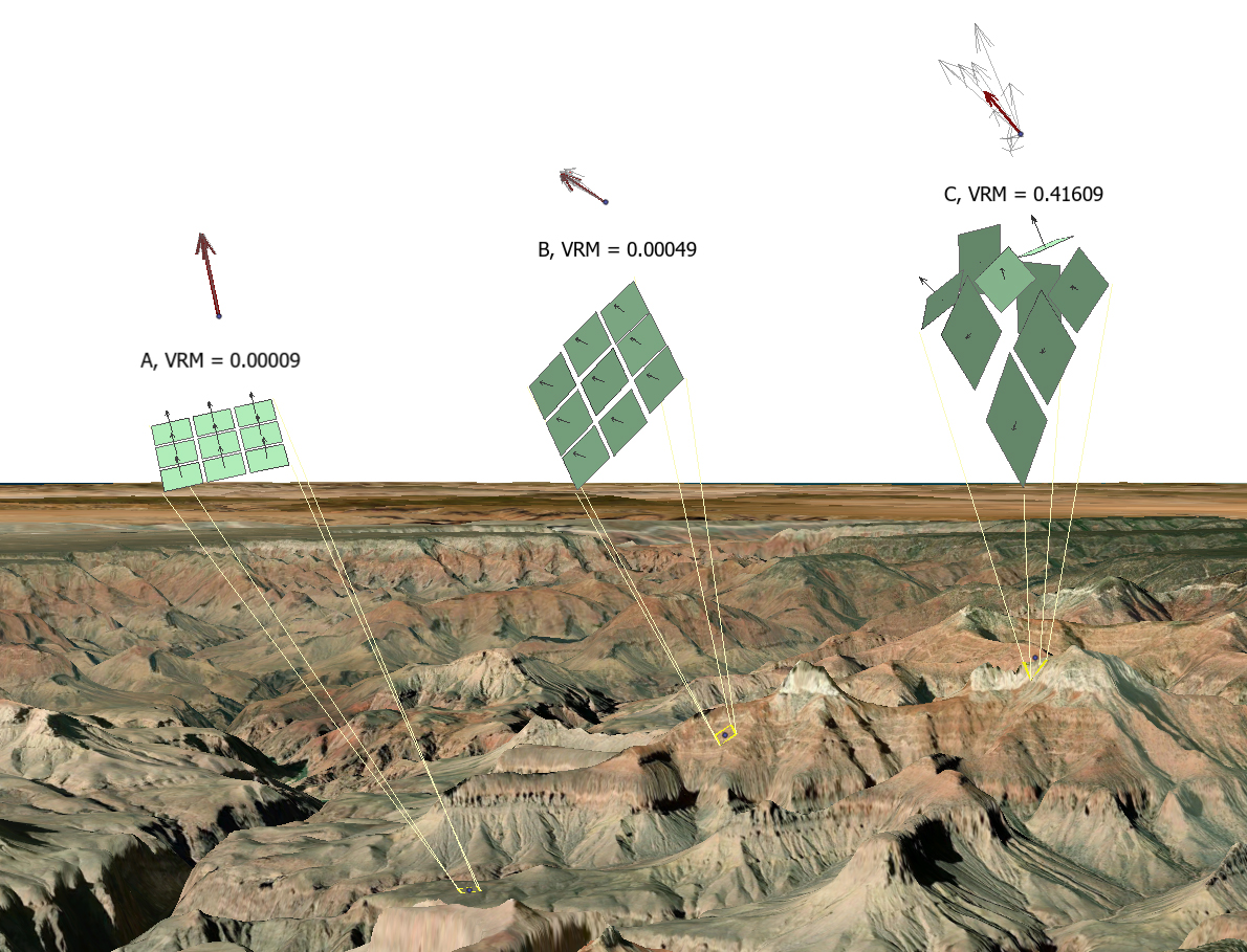
The figure above shows the idea on real ground. At A the nine cells are nearly level and their normals all point straight up. At B the cells are steep, but they are all steep in the same direction, so their normals are just as parallel as at A; they simply lean. At C the cells face every which way. Now look at the little bundles of arrows above each block, where the nine normals have been gathered to a common origin. At A and B the nine arrows lie so nearly on top of one another that they look like one, and the red resultant is as long as it can be. At C they splay apart and the resultant is little more than half as long. VRM is nothing more than that shortfall: 0.00009 at A, 0.00049 at B and 0.416 at C. The even 42° slope and the nearly level ground are, to VRM, the same kind of ground, and that is the whole point of the measure.
From compass directions to a sphere
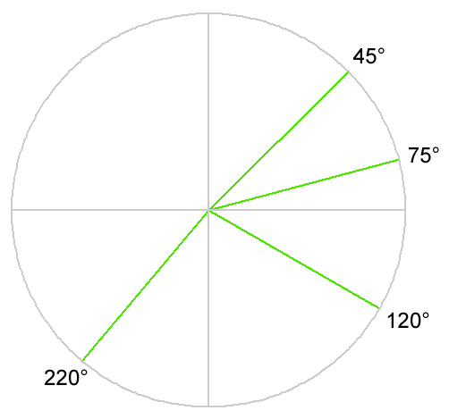
VRM is easiest to understand by starting with ordinary compass directions, because it is the same statistic moved from a circle onto a sphere. Suppose we have four directions and want a single number describing how much they disagree. Draw each direction as an arrow of length one, then string the arrows end to end, in any order, into a path. The straight line from the start of the path to its end is the resultant, and its length tells us how much the arrows reinforced one another. If all four pointed the same way, the path would be a straight line four units long. If they pointed in every direction, the path would wander back toward where it started and the resultant would be short.
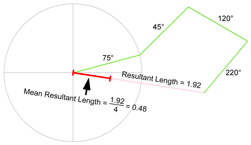
Dividing the resultant length by the number of arrows gives the mean resultant length, which Fisher (1993) writes as . It is 1 when every direction is the same and 0 when they cancel out completely. For our four directions the resultant is 1.92 and the mean resultant length is 1.92 / 4 = 0.48. Most people do not use the mean resultant length directly; they subtract it from 1 to get the circular variance, so that 0 means perfect agreement and values near 1 mean high dispersion. Here the circular variance is 1 − 0.48 = 0.52.
One caution from the compass version carries straight over to the terrain version. A mean resultant length near 0 can mean the directions are scattered everywhere, but it can also mean they are balanced in opposing pairs: an animal that commutes from a roost to a foraging area and straight back has only two headings, yet its resultant is zero. Fisher (1993) makes the same point with a data set that has well-defined modal groups and yet a mean resultant length of effectively zero. On terrain, this is why a knife-edge ridge scores high: the cells on its two faces point in opposite directions and largely cancel, exactly as though the surface were scattered, and that is the smooth-fold problem the detrending option below is meant to address.
The vector in each cell
A compass direction is a point on a circle. The direction a piece of ground faces is a point on a sphere, and it takes a three-dimensional unit vector to describe it: the vector that stands perpendicular to the cell's surface, called the normal vector. On a flat cell the normal points straight up. As the cell tilts, the normal leans over in the direction of the aspect, and the steeper the cell, the further it leans. Sappington et al. decompose that vector into its three components from the cell's slope and aspect :
so that a flat cell is (0, 0, 1); a cell tilted 20° and facing due east is (sin 20°, 0, cos 20°) = (0.342, 0, 0.940); and a cell tilted 20° and facing due west is (−0.342, 0, 0.940). The length of every one of these vectors is exactly 1, which is the point: each cell gets one vote, and the vote records only direction. This tool does not go through slope and aspect at all. It computes the normal directly from the east-west and north-south gradients of Horn's method (Horn 1981), the same gradients that underlie the ArcGIS Slope tool, using true ground distances at each row's latitude. The resulting vector is the same one Sappington's trigonometry produces, only expressed without the detour through angles, and because VRM depends only on the length of the sum of the vectors, the two are interchangeable. Computing a cell's own normal needs its full 3 × 3 window, so each VRM value depends on elevations up to one cell beyond your chosen radius; along the DEM's outer edge, VRM is computed from the normals that exist.
Computing VRM
With a unit vector for every cell, VRM within a neighborhood of cells is the compass calculation done in three dimensions. Add up the components, the components and the components separately, take the length of the resultant, divide by the number of vectors, and subtract from 1:
Three small examples show how it behaves. Take five cells that all tilt 20° and all face north: every vector is (0, 0.342, 0.940), the sums are (0, 1.710, 4.698), the resultant is exactly 5, and VRM = 1 − 5/5 = 0. The neighborhood is steep but perfectly even, and VRM says so. Now let the five cells tilt 20° toward north, east, south and west, with the fifth flat. The horizontal components cancel in pairs, the vertical components add to 4 × 0.940 + 1 = 4.759, the resultant is 4.759, and VRM = 1 − 4.759/5 = 0.048. Finally, take a full 3 × 3 window in which the eight surrounding cells tilt 45° toward the eight compass points and the center is flat, a little pyramid: the resultant is 6.657 and VRM = 1 − 6.657/9 = 0.260. These numbers illustrate something you will see on real DEMs: VRM values are small. Even that pyramid, a thoroughly broken 3 × 3 window, reaches only 0.26, and values above 0.5 are rare: on the Grand Canyon DEM used in the examples below, 0.45% of the cells are above 0.2 and 0.0004% are above 0.5. The theoretical maximum of 1 requires the normals to cancel completely, which a DEM surface never can, since every normal has an upward component. Sappington et al. found that values on natural terrain were rarely above 0.2 and that the mean VRM in each of their three mountain ranges was about 0.01, with a long right tail; they could push values above 0.8 only on artificial terrain. So do not be alarmed when your VRM raster is full of numbers like 0.004; small values are what the measure produces. They are nonetheless real, comparable numbers. VRM is dimensionless and has a fixed meaning (one minus the mean resultant length of the normals), so a value of 0.05 describes the same amount of directional scatter wherever it occurs, and Sappington et al. themselves compared mean ruggedness among their three ranges (0.0112 in the Black Mountains, 0.0108 in the Eagle Mountains and 0.0077 in the Eldorado Mountains). You can use VRM in either way: as a relative measure, ranking locations within one landscape, or as an absolute one, comparing landscapes with each other. The absolute comparison is fair only when the two rasters were computed the same way, from DEMs of the same cell size and with the same neighborhood radius, because both of those change the values.
The neighborhood
The neighborhood is a circle centered on each cell, with a radius you set in cells or in ground units (meters, kilometers, feet or miles). Ground-unit radii are converted to cells from the cell size. On a geographic DEM the conversion is done row by row on the spheroid, with the east–west radius rounded to a whole number of cells for each row (the north–south radius is exact), so the circle stays close to the right size on the ground at any latitude; for small ground-unit radii the rounding can be a sizable fraction of the radius, and giving the radius in cells avoids it. The same rounding applies to the detrending radius here and in the Surface Area and Arc-Chord Ratio tools; the Terrain Ruggedness Index tool uses an exact per-row mask instead. Sappington's original neighborhood was a 3 × 3 square: the focal cell and its eight neighbors, about 8,100 m² on their 30 m DEM. To reproduce it with a circle, use the default radius of 1.5 cells. The four diagonal neighbors sit √2 ≈ 1.41 cells from the center, so a radius of 1.5 takes in all eight, whereas a radius of exactly 1 cell includes only the four orthogonal neighbors and gives a five-cell plus shape. Larger radii measure ruggedness at a coarser landscape scale. There is no fixed relationship between the radius and the size of the VRM values, since a larger window can take in more terrain diversity rather than less, but Sappington et al. did find that larger neighborhoods smoothed the landscape for their purposes, which is one of their two reasons for staying with 3 × 3 (the other was to keep VRM comparable with the two indices they tested it against). There's no law that says you can't try two or three radii and look at the results before settling on one.
The neighborhood aggregation ignores NoData rather than propagating it: VRM is computed wherever at least one valid normal vector falls within the radius, even where the focal cell's own elevation is NoData, so a small gap in the DEM is filled in from the cells around it. Cells with no valid neighbor vector at all are NoData in the output.
Local detrending: VRM-L
VRM passes the first of the three tests Dilts et al. (2023) apply to a ruggedness index, independence from slope, but not the second. A smooth fold, such as a rounded ridgeline or the bottom of a gentle drainage, reads as rugged because the cells on either side of it face different directions even though the surface itself is perfectly smooth; the knife-edge ridge above is the extreme case. On the synthetic surfaces of Dilts et al. a tilted plane gave a VRM of exactly zero, while on smooth sinusoidal folds VRM crept above zero only on the most tightly folded surface (0.0005), enough for them to class it as failing. On real Nevada terrain the effect was larger: with VRM-L in place of VRM, 45% fewer drainage cells and 46% fewer ridge cells fell in the most rugged tenth of the landscape. Their fix is a simple pre-processing step. Turn on Remove smooth topography first and the tool smooths the DEM with a circular neighborhood mean of the radius you set (the default, 1.5 cells, is exactly the 3 × 3 mean they used), subtracts that smoothed surface from the original, and computes VRM on what is left. The residual holds only the variation finer than the smoothing radius: the slope is gone, the fold is gone, and only the bumps remain. The result is what Dilts et al. call VRM-L, the local variant, which passed all three of their criteria for an ideal index (independent of slope, unaffected by smooth folding, and rising only with true surface roughness) and modestly improved their bighorn sheep habitat models (McFadden's R² rose by 0.020).
The detrending radius and the VRM radius are separate settings and play different roles. The detrending radius decides how large a feature counts as smooth topography to be removed; the VRM radius decides over how wide an area the remaining roughness is summarized. Dilts et al. computed VRM at twenty-one spatial scales, from 30 m to 1,230 m, but always detrended with the same 3 × 3 mean. A larger detrending radius leaves broader features in the residual, so hills a few cells across count as roughness at a 10-cell detrending radius and disappear at 1.5.
Geographic DEMs and elevation units
The gradients that define each cell's normal are computed from true spheroidal distances at every row's latitude, so the tool is correct on a geographic (latitude/longitude) DEM without projecting it first, and you avoid the resampling that projection imposes on a raster (see Projecting Rasters). The elevation units matter because the normal vector combines a vertical difference with a horizontal distance: a DEM in feet treated as meters would tilt every normal too far and inflate the roughness. The tool reads the units from the DEM's vertical coordinate system when it has one and locks the setting, assumes meters for geographic DEMs, and asks you only when the DEM does not say.
A tour of the dialog
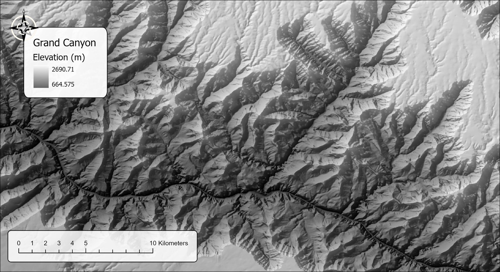
The example uses the same 30 m DEM of the Grand Canyon as the Surface Area and Ratio page, so you can compare the two measures on identical ground: about 2,000 m of relief, smooth plateaus on both rims, and walls built of stacked cliff bands cut by many side drainages.
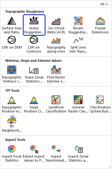
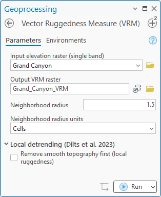
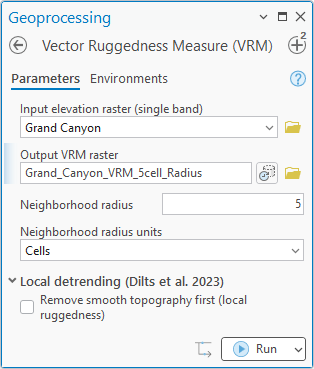
The dialog asks for the DEM, an output name (suggested from the input), and the neighborhood radius and its units. The detrending options sit in their own collapsible category. An Elevation units row appears only when the tool cannot work the units out for itself; here it could, so the row is absent. That is the whole dialog: VRM has no method choices, because the measure itself is fixed, and the neighborhood radius is the one decision that changes what you get.
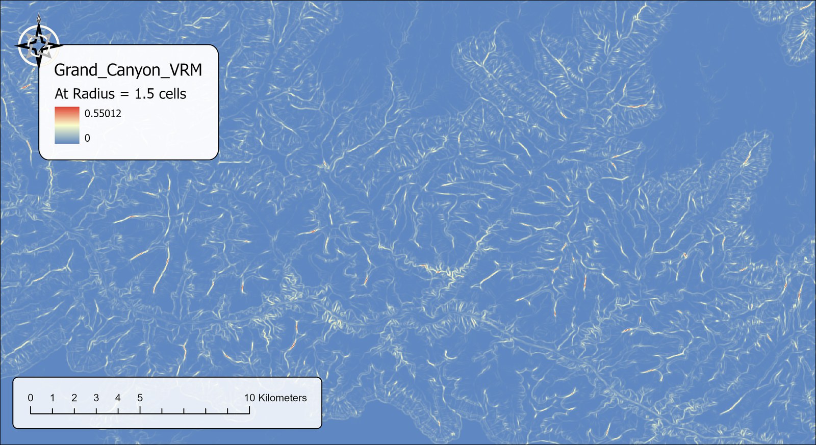
Two things are worth noticing in that map. First, the maximum of 0.55 is far above the 0.2 that Sappington et al. rarely saw exceeded; as on the Surface Area page, that is the Grand Canyon being the Grand Canyon, and the high values are confined to a tiny share of the cells (fewer than half a percent exceed 0.2). Second, look at what kind of feature scores high. A great many of those bright lines are drainage bottoms and ridge crests whose flanks may be quite smooth. They score high because one flank faces east and the other west, which is the smooth-fold problem described above, and it is exactly what the detrending option is for.
VRM-L: the same run with detrending
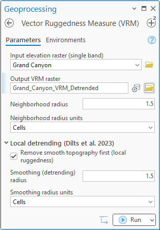
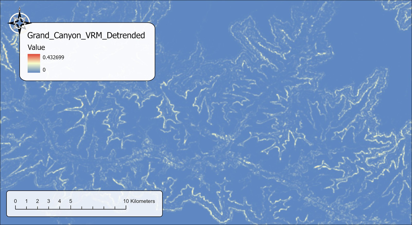
It helps to be clear about the order of operations, because the name of the option describes it literally. Detrending is a separate first pass over the whole DEM. The tool computes the neighborhood mean of every cell at the smoothing radius, subtracts that smoothed surface from the original, and writes the residual to a temporary raster: a DEM of bumps and hollows around zero, with the canyon itself removed. Only then does the ordinary VRM computation run, start to finish, on that residual raster exactly as it would on any DEM. Nothing about the VRM arithmetic changes; it is simply given a different surface to work on. That is also why the smoothing radius and the VRM radius are independent settings: one shapes the surface, the other summarizes it.
The same canyon at three radii
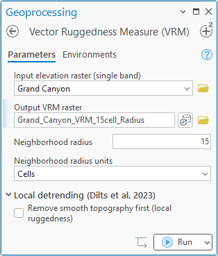
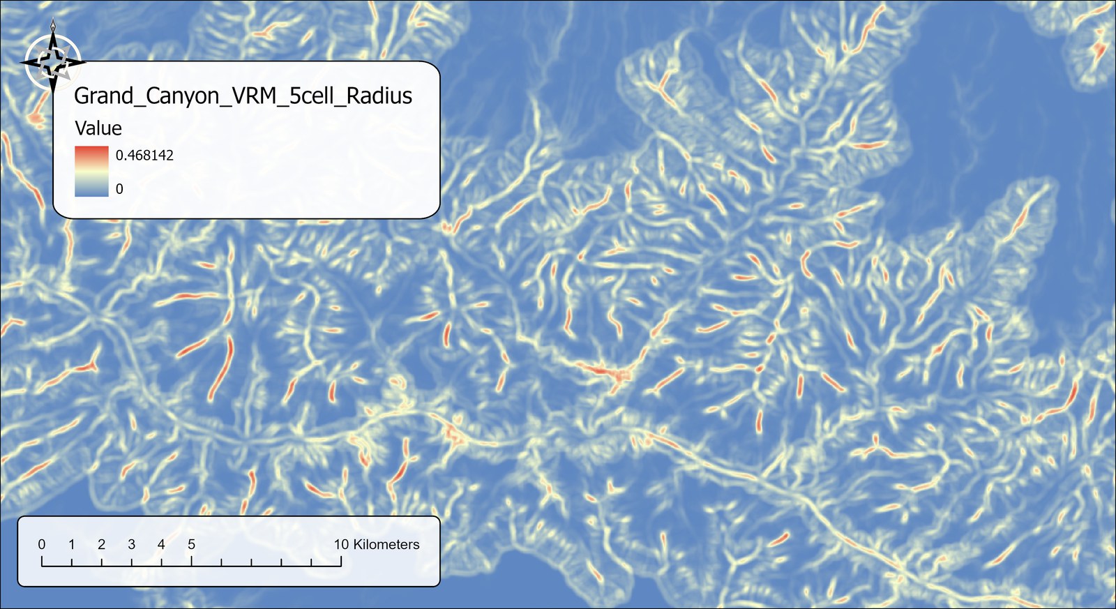
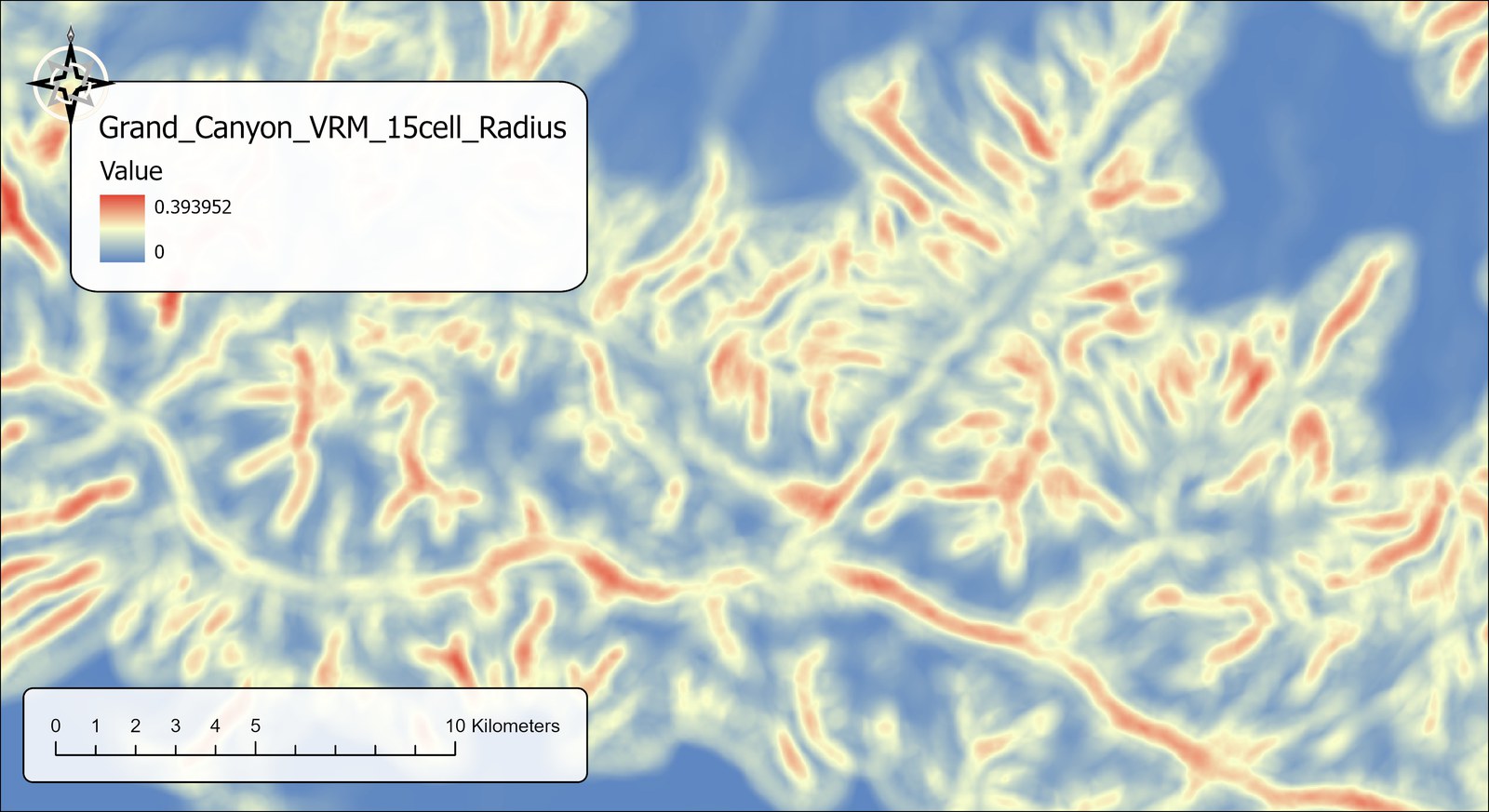
These three maps (1.5, 5 and 15 cells) are the same measure on the same DEM, and they answer three different questions. At 1.5 cells VRM finds individual edges a few tens of meters across. At 5 cells it describes the ground within about 140 m of each cell, roughly a football field and a half, which is the scale of a single cliff band or side ravine. At 15 cells, a radius of about 420 m, it describes whole side canyons and the inner gorge. Which of those scales matters depends on the animal and the question, and that is a judgment for you to make from what is known about the species. Notice also what happens to the numbers: the maximum falls steadily, from 0.55 to 0.47 to 0.39, while the amount of the map that is not blue grows. On this DEM the maximum falls as the radius grows, because the sharpest breaks are averaged with their smoother surroundings, while every rough feature's influence is spread over a wider area. That is not a rule: in a V-shaped valley with smooth 45° walls, the 3 × 3 window at the bottom scores 0.195, and a wide window spanning both walls scores 0.293, higher than any 3 × 3 window inside it. What happened on this DEM is the smoothing effect Sappington et al. described, and it is the reason VRM values from different radii should never be compared with one another.
The output is a floating-point raster of values from 0 to 1, with statistics, a histogram and bilinear pyramids already built, so it draws correctly the moment it reaches the map, and a blue-yellow-red stretch is applied by default. Outputs may go into a geodatabase or a folder; in a folder a name without an extension becomes a GeoTIFF.
The tool holds the whole DEM in memory at once, so the memory it needs grows with the number of cells. On most DEMs that is no concern. On a very large one the tool may need more memory than your computer has free, and then one of two things happens: Windows starts using the disk as overflow memory and the tool slows to a crawl, or the tool stops with an out-of-memory error. There is no fixed limit; it depends on how much memory your computer has free. If a DEM is too large, clip it to the area you need first.
Environment settings
The output matches the input DEM exactly: same extent, cell size and coordinate system. The Processing Extent, Snap Raster, Cell Size, Output Coordinate System and Mask environments are deliberately not applied, so that the delivered raster is the grid the VRM values were computed on; project, clip or resample the finished raster yourself if you need to. Pyramids are always built with bilinear resampling regardless of the Pyramid environment.
ModelBuilder
Parameters
| Label | Explanation | Data type |
|---|---|---|
| Input elevation raster (single band)Required · in_raster | The DEM. Must be single band; projected or geographic. Choose a layer from the map or browse to a dataset. | Raster Layer |
| Output VRM rasterRequired · out_raster | Floating point, 0 to 1; NoData where no valid normal vector falls within the neighborhood. A name is suggested from the input. | Raster Dataset |
| Elevation unitsOptional · elev_units | Meters or Feet. Filled in and locked from the DEM's vertical coordinate system when it has one; geographic DEMs are assumed to be in meters; you are asked only when the DEM does not say. | String |
| Neighborhood radiusRequired · radius | How far the circular neighborhood extends around each cell. The default 1.5 cells reproduces Sappington's 3 × 3 neighborhood; larger values measure ruggedness at a coarser scale. | Double |
| Neighborhood radius unitsRequired · radius_units | Cells, Meters, Kilometers, Feet or Miles. Ground units are converted to cells from the cell size, per row on the spheroid for geographic DEMs. | String |
| Remove smooth topography first (local ruggedness)Optional · detrend | Subtract a circular neighborhood mean of the DEM before computing, giving the local variant VRM-L of Dilts et al. (2023). Off by default. | Boolean |
| Smoothing (detrending) radiusOptional · detrend_radius | Radius of the smoothing mean. The default 1.5 cells is exactly a 3 × 3 mean; larger radii remove broader topography. Used only when detrending is on. | Double |
| Smoothing radius unitsOptional · detrend_units | Cells, Meters, Kilometers, Feet or Miles, converted to cells like the neighborhood radius, including the whole-cell rounding per row on a geographic DEM. Used only when detrending is on. | String |
Python
import arcpy
arcpy.ImportToolbox(r"C:\path\to\JennessEnterprisesTools.pyt")  # your install path
# VRM at Sappington's 3 x 3 scale.
arcpy.jenness.VRM(
    in_raster=r"C:\Project\Elev.gdb\DEM",
    out_raster=r"C:\Project\Elev.gdb\DEM_VRM_3x3",
    elev_units="Meters", radius=1.5, radius_units="Cells")
# The local (detrended) variant VRM-L, with a 3 x 3 smoothing mean.
arcpy.jenness.VRM(
    in_raster=r"C:\Project\Elev.gdb\DEM",
    out_raster=r"C:\Project\Elev.gdb\DEM_VRML",
    elev_units="Meters", radius=1.5, radius_units="Cells",
    detrend=True, detrend_radius=1.5, detrend_units="Cells")
Recommended citation
Credits and references
By Jeff Jenness, Jenness Enterprises (www.jennessent.com), modernizing the Vector Ruggedness Measure function of his DEM Surface Tools extension for ArcGIS 9.x, which in turn implemented the method and ArcView script of Sappington, Longshore and Thompson (2007). The local-detrending option follows Dilts et al. (2023).
- Beasom, S. L., E. P. Wiggers, and J. R. Giardino. 1983. A technique for assessing land surface ruggedness. Journal of Wildlife Management 47:1163–1166. doi.org/10.2307/3808184
- Dilts, T. E., M. E. Blum, K. T. Shoemaker, P. J. Weisberg, and K. M. Stewart. 2023. Improved topographic ruggedness indices more accurately model fine-scale ecological patterns. Landscape Ecology 38:1395–1410. doi.org/10.1007/s10980-023-01646-6
- Fisher, N. I. 1993. Statistical Analysis of Circular Data. Cambridge University Press, Cambridge. Section 2.3. doi.org/10.1017/CBO9780511564345
- Hobson, R. D. 1972. Surface roughness in topography: quantitative approach. Pages 221–245 in R. J. Chorley, editor. Spatial Analysis in Geomorphology. Harper & Row, New York.
- Horn, B. K. P. 1981. Hill shading and the reflectance map. Proceedings of the IEEE 69:14–47. doi.org/10.1109/PROC.1981.11918
- Jenness, J. 2013. DEM Surface Tools for ArcGIS (v. 2.1.375). Jenness Enterprises. jennessent.com/arcgis/surface_area.htm
- Riley, S. J., S. D. DeGloria, and R. Elliot. 1999. A terrain ruggedness index that quantifies topographic heterogeneity. Intermountain Journal of Sciences 5:23–27. download.osgeo.org/qgis/doc/reference-docs/Terrain_Ruggedness_Index.pdf
- Sappington, J. M., K. M. Longshore, and D. B. Thompson. 2007. Quantifying landscape ruggedness for animal habitat analysis: a case study using bighorn sheep in the Mojave Desert. Journal of Wildlife Management 71:1419–1426. doi.org/10.2193/2005-723
Licensing information
Works at every ArcGIS Pro license level (Basic, Standard, Advanced). No extension licenses are required; the gradients, normal vectors and neighborhood sums are computed internally, without Spatial Analyst.
Related tools and pages
- About Topographic Roughness — choosing among the nine roughness measures, and the three generations of ruggedness index.
- Arc-Chord Ratio (ACR) — the other second-generation index, which removes slope from the surface ratio instead.
- Terrain Ruggedness Index (TRI) — the elevation-difference indices that VRM was designed to complement.
- Surface Area and Ratio — roughness as extra land surface, correlated with slope by design.
- Fractal Dimension — the other slope-independent measure, describing roughness across scales.
- Projecting Rasters — why this tool works on geographic DEMs directly.