

Enhanced Hillshade
Summary
Computes a hillshade from a single-band DEM with one sun, as ArcGIS Pro's own Hillshade tool does, but with four things Pro's tool lacks. It can darken the low elevations for the atmospheric-perspective effect of the Swiss method. Its cast shadows, if you ask for them, are dimmed rather than black, so the relief stays visible inside them. It lets you choose the number of gray levels, so you can make a smooth 256-level hillshade or a posterized one with a handful of tones. And it is correct on latitude/longitude DEMs without projecting them, because the ground dimensions of the cells are recomputed for every row from the spheroid. A vertical-exaggeration factor rounds out the options. The tool needs no Spatial Analyst license.
What the tool does
The hillshade is the standard one: for each cell the slope and aspect are found from the eight neighbors with Horn's (1981) equations, and the brightness is the cosine of the angle between the sun and the surface normal (i.e. the direction into the sky that is perpendicular to the ground at that location), automatically set to zero (fully shaded) for ground that faces away from the sun and divided into the number of gray levels you ask for. With 256 levels and a projected DEM in meters the result matches the familiar Esri hillshade, to within one gray level. The About Hillshades page gives the formula. Everything else on this page is about the four enhancements.
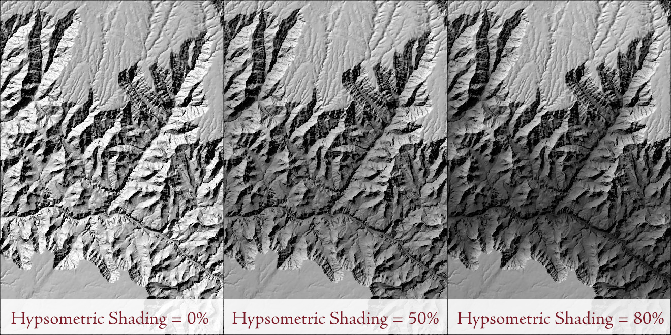
Hypsometric shading
The atmospheric-perspective component of the Swiss method. With Apply hypsometric shading checked, every cell's hillshade value is multiplied by a factor that depends on its elevation: at a strength of s percent the factor is (100 − s) percent at the lowest elevation in the DEM and rises in a straight line to 100 percent at the highest. At the default strength of 50 the valley floors are half as bright as they would otherwise be and the summits are untouched. The elevation range used is that of the whole DEM, so on a DEM that extends far beyond your map the effect can be slight within the area you are looking at; clip the DEM to your area first if that happens. (Setting the Processing Extent does not help: the tool takes the elevation range from the whole DEM and applies the extent afterward.) The Simple Hypsometric Shading tool provides you with a similar effect from layers alone, and stays adjustable afterward.
Cast shadows that keep their detail
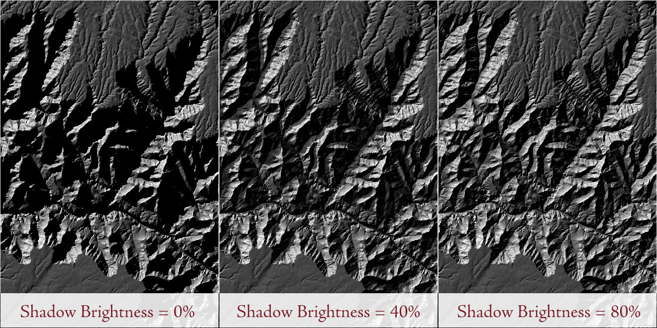
A hillshade on its own lights every cell as if nothing stood between it and the sun. Real terrain casts shadows: a slope that faces the sun squarely may still lie in the shade of a higher ridge. Esri's Model shadows option finds those cells and sets them to 0, solid black. This tool finds them and instead dims them to a percentage of their unshadowed value, the Shadow brightness. At the default 20 percent the shadows are dark but the terrain inside them can still be made out; at 0 percent they are black, as in Esri's tool; at 100 percent the option does nothing.
The shadows are found with a single sweep across the grid in the direction the shadows fall, carrying along the height of the shadow-casting surface and dropping it by the tangent of the sun's altitude at each step, rather than by tracing a ray back toward the sun from every cell. That makes the option fast even on large DEMs, a matter of seconds for tens of millions of cells, but it needs the entire DEM in memory at once, unlike the hillshade itself, which is computed in strips.
That difference matters on a very large DEM. A calculation done in strips uses about the same modest amount of memory however large the DEM is, while the shadow sweep uses memory in proportion to the number of cells, about 25 bytes per cell at its peak. A DEM of 10,000 by 10,000 cells (100 million cells) therefore needs about 2.5 gigabytes, which most computers can spare. A DEM of a billion cells, roughly 32,000 by 32,000, needs about 25 gigabytes, which is more than many computers have free. Past what your computer can spare, one of two things happens: Windows starts using the disk as overflow memory and the tool slows to a crawl, or the tool stops with an out-of-memory error. There is no fixed limit, then; it depends on how much memory your computer has free. If a DEM is too large for the shadow option, clip it to the area you need, or run the tool without shadows, which is not limited in this way.
On a geographic DEM the sweep uses the mean cell dimensions of the raster, an approximation the tool notes in its messages; the hillshade itself remains exact row by row. The tool reports how many cells it found in shadow.
Hillshade gray levels
Esri's hillshade runs from 0 to 255 because that is the numeric range of an 8-bit raster. There is otherwise nothing special about that range of numbers. This tool divides the range from fully shaded to fully lit into as many equal gray levels as you ask for, numbered from 0: 256 for the standard look (values 0 to 255), a larger number if you want finer gradations (though they are unlikely to be visible on a screen), or a small number for a deliberately posterized hillshade in which the terrain is drawn in a few flat tones, an effect some cartographers like for stylized maps. Ask for 3 levels and the output holds exactly three values, 0, 1 and 2: the darkest third of the illumination range, the middle third and the brightest third.
When you ask for 32 or fewer levels, the output also gets a raster attribute table, with one row for each gray level present and the number of cells it covers. That makes a posterized hillshade easy to symbolize with unique values, or to summarize. A full-range hillshade is not given a table, since a list of 256 gray values is rarely useful and building it takes an extra pass through the raster. If you need a table for that raster, you can always use Esri's “Build Raster Attribute Table” option to create it yourself.
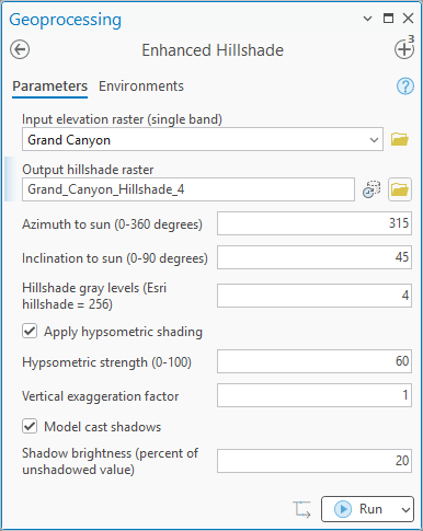
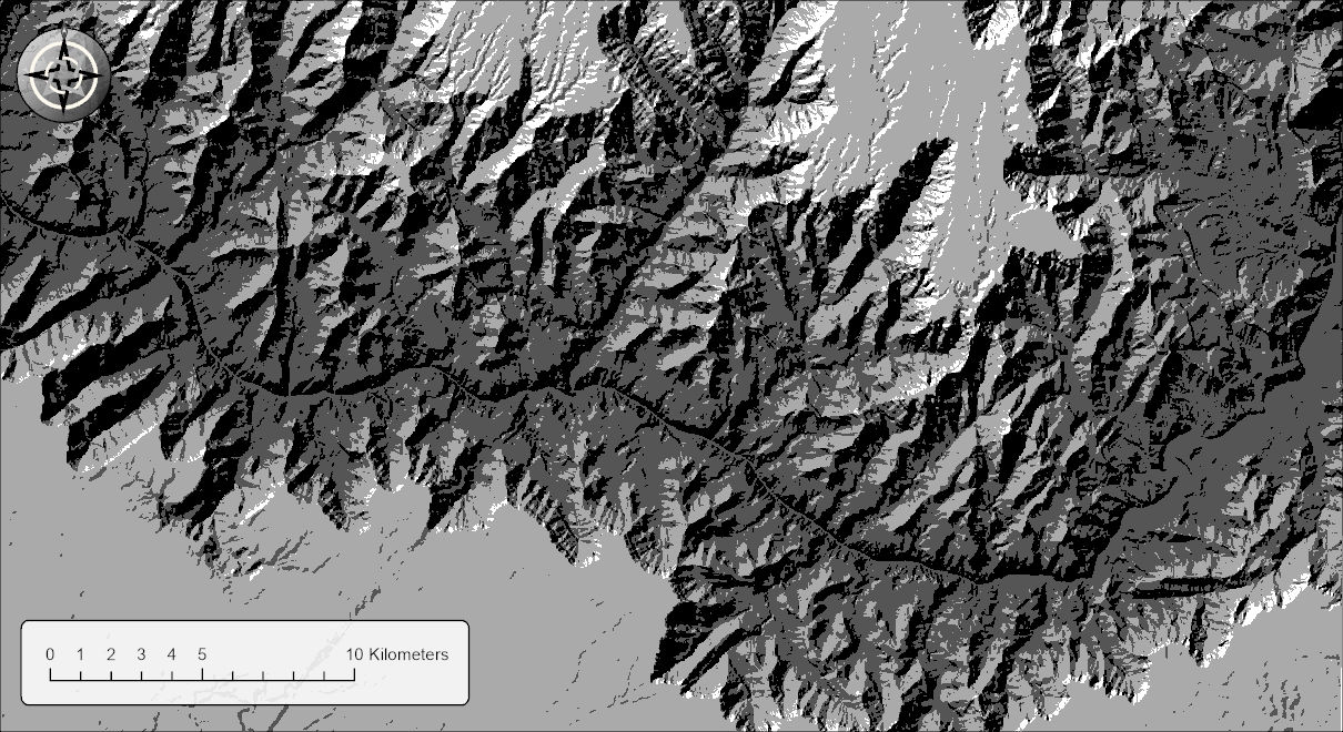
The pane and the hillshade below are a posterized run: the same settings as the full-range hillshade shown under A tour of the dialog, with Hillshade gray levels set to 4.
Correct on geographic DEMs
A DEM in geographic coordinates has cells that are a fraction of a degree on a side, and a degree of longitude is a different number of meters at every latitude. Pro's Hillshade tool, given such a DEM, either produces nonsense or has to be handed a Z factor that converts meters into approximate degrees for the latitude of the middle of the raster, an approximation that gets worse toward the top and bottom of a tall DEM. This tool instead computes the true east-west and north-south ground distances between cell centers for every row from the spheroid's dimensions, and uses those distances in the gradient, so the slopes and the shading are right at every latitude. A projected DEM is handled with the ordinary constant-cell formulas, which are faster. On a projected DEM whose linear unit is feet, the horizontal distances are converted to meters automatically.
The elevation units matter as well, since a gradient is a rise over a run and the two must be in the same units. The tool reads the units from the DEM's vertical coordinate system when it has one and hides the Elevation units setting; a geographic DEM that does not say is assumed to be in meters, which is the usual case; and only when the DEM gives no hint at all are you asked to choose meters or feet. A DEM in feet is scaled by 0.3048.
Vertical exaggeration
Multiplies the elevations before the shading is computed. A factor of 2 makes gentle country look twice as steep, which can bring out relief on a plain that a plain hillshade leaves nearly blank; a factor of 0.5 tones down a mountain range. It changes only the picture; nothing about the DEM is altered.
A tour of the dialog
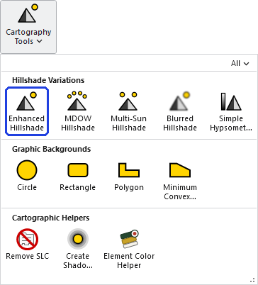
The tool opens from the Cartography group of the Wildlife and Forestry Tools ribbon tab or from the Cartography Tools toolset of the Jenness Enterprises toolbox; either way it is the same geoprocessing tool, and it works in ModelBuilder.
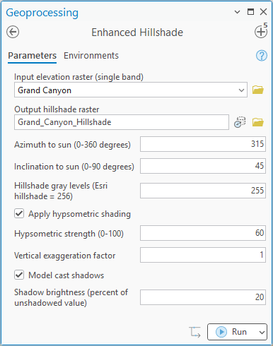
Choose the DEM from the map or browse to one; it must be single band. An output name is suggested from the input. The Elevation units row appears only when the tool cannot tell what the elevation units are; when the DEM declares its vertical units, or is in geographic coordinates, the tool settles the units itself and Pro hides the row, as in the pane above. Then the sun: azimuth in compass degrees, 315 by default, and inclination above the horizon, 45 by default (if you wonder why we put the sun in a location it rarely actually sits in the sky, see the discussion on Why the sun is always in the northwest on the About Hillshades page). Next specify how many shades of gray you want (50 shades of gray is a perfectly valid choice). The hypsometric option and its strength, the exaggeration factor, and the shadow option and its brightness are all optional and off, or at 1, by default. The Hypsometric strength and Shadow brightness rows appear only when their boxes are checked. Your last choices are remembered with the project.
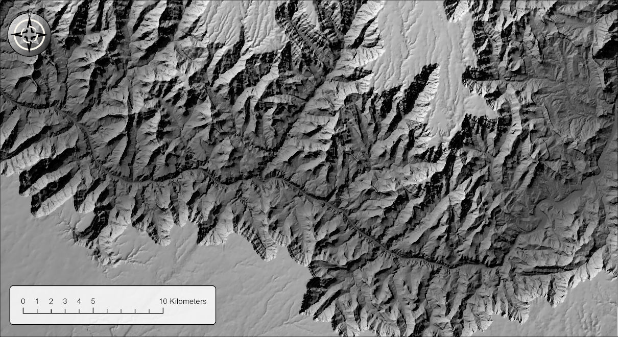
The output is a 16-bit integer raster, from 0 to one less than the number of gray levels, with statistics, a histogram and bilinear pyramids already built, and Pro draws it with a black-to-white stretch in which white is the highest value actually present. An output with 32 or fewer gray levels is drawn with unique values instead, one gray for each level present, from black for 0 to white for the highest. It may go into a geodatabase or a folder; in a folder a name without an extension becomes a GeoTIFF.
Environment settings
By default the output matches the input DEM exactly: same extent, cell size and coordinate system. Processing Extent, Snap Raster, Cell Size and Output Coordinate System are honored, all as finishing steps applied to the computed hillshade: the shading is computed from the full-resolution DEM first and the finished raster is then clipped (with the snap raster aligning the window), resampled, or reprojected. Cells at a clipped edge therefore carry true hillshade values, and resampling smooths the finished picture rather than recomputing it on a coarser grid. The Mask environment is not honored, and pyramids are always built with bilinear resampling regardless of the Pyramid environment.
ModelBuilder
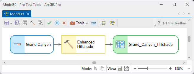
In a model the tool takes one input, the DEM, and produces one output, the hillshade raster, which can go on to any tool that takes a raster.
Parameters
| Label | Explanation | Data type |
|---|---|---|
| Input elevation raster (single band)Required · in_raster | The DEM. Must be single band; projected or geographic. Choose a layer from the map or browse to a dataset. | Raster Layer |
| Output hillshade rasterRequired · out_raster | The hillshade (integer, 0 to one less than the number of gray levels). NoData where the DEM is NoData and at its outer edge. A name is suggested from the input. | Raster Dataset |
| Elevation unitsOptional · elev_units | Meters or Feet. Read from the DEM's vertical coordinate system when it has one; geographic DEMs are assumed to be in meters. In both cases the row is hidden in the dialog; you are asked only when the DEM does not say. | String |
| Azimuth to sun (0-360 degrees)Required · azimuth | The compass direction of the sun, clockwise from north. The default 315 (northwest) is the cartographic convention. | Double |
| Inclination to sun (0-90 degrees)Required · altitude | The height of the sun above the horizon, from 0 (grazing) to 90 (overhead). The default is 45. | Double |
| Hillshade gray levels (Esri hillshade = 256)Required · levels | The number of gray levels; output values run from 0 to one less than this number. The default 256 matches the standard Esri hillshade; a small number posterizes, and 32 or fewer adds a raster attribute table. | Long |
| Apply hypsometric shadingOptional · use_hypso | Darkens low elevations by the strength below. Off by default. | Boolean |
| Hypsometric strength (0-100)Optional · hypso_strength | At strength s, the brightness multiplier runs from (100 − s) percent at the lowest elevation to 100 percent at the highest. The default is 50. | Long |
| Vertical exaggeration factorOptional · vert_exag | Multiplies the elevations before shading. The default is 1. | Double |
| Model cast shadowsOptional · model_shadows | Dims ground hidden from the sun behind higher terrain to the brightness below. Needs the whole DEM in memory. Off by default. | Boolean |
| Shadow brightness (percent of unshadowed value)Optional · shadow_dim | What a shadowed cell keeps of its unshadowed value: 0 for black shadows, larger to keep detail inside them. The default is 20. | Double |
Python
import arcpy
arcpy.ImportToolbox(r"C:\path\to\JennessEnterprisesTools.pyt")  # your install path
# A geographic DEM, hypsometric shading at 40 percent, soft cast shadows.
arcpy.jenness.EnhancedHillshade(
    in_raster=r"C:\Project\Elev.gdb\DEM_WGS84",
    out_raster=r"C:\Project\Elev.gdb\DEM_Hillshade",
    elev_units="Meters", azimuth=315, altitude=45, levels=256,
    use_hypso=True, hypso_strength=40, vert_exag=1,
    model_shadows=True, shadow_dim=20)
Recommended citation
Credits and references
By Jeff Jenness, Jenness Enterprises (www.jennessent.com). A port of the hillshade function in the author's DEM Surface Tools for ArcGIS (Jenness 2013), with the shadow option rewritten. The gradient is Horn's (1981).
- Horn, B. K. P. 1981. Hill shading and the reflectance map. Proceedings of the IEEE 69:14–47. doi.org/10.1109/PROC.1981.11918
- Jenness, J. 2013. DEM Surface Tools for ArcGIS (v. 2.1.375). Jenness Enterprises. jennessent.com/arcgis/surface_area.htm
- Jenness, J. Raster lab 3: Calculating hillshades from a DEM in ArcGIS Pro. Lab exercise video, GIS training courses, Jenness Enterprises. youtu.be/Eduy5QAoLE0
Licensing information
Works at every ArcGIS Pro license level (Basic, Standard, Advanced). No extension licenses are required; the gradients, shading and shadows are computed internally, without Spatial Analyst.
Related tools and pages
- About Hillshades and the Swiss Method — the formula, the northwest sun, and the five tools compared.
- MDOW Hillshade — four suns, weighted by aspect.
- Multi-Sun Hillshade — a weighted average of suns you place; every option here plus per-sun shadows.
- Blurred Hillshade — every option here plus a blur.
- Simple Hypsometric Shading — the hypsometric effect as an adjustable group layer.
- Projecting Rasters — this tool works on geographic DEMs directly; if you project a DEM first, use bilinear interpolation.