

Random Point Generator
Summary
Generates uniform random points inside polygon features (selection honored, holes respected), along polyline features, within the data cells of an integer raster's categories, or in a plain extent — with two optional hard constraints Esri's random-point tools do not offer together: a minimum separation between points, and a minimum separation from the area boundary. Stratified designs follow the same model as Esri's Create Spatial Sampling Locations: strata are individual polygons or polylines, raster categories, contiguous raster regions, or groups sharing a strata ID value, and counts are allocated equally, proportionally to stratum area or length, from a population field, or by density in real units. An optional seed makes runs exactly reproducible.
A modernized port of the classic Random Point Generator extension — the workhorse for drawing statistically defensible field designs: accuracy-assessment samples over a classified raster, survey stations along stream networks, or plots inside study-area polygons.
Usage
Random sampling is the price of admission to inferential statistics: points placed by judgment tell you about those points, while points placed at random let the sample speak for the whole landscape. This tool draws that sample — uniformly, stratified, or constrained by spacing rules — and does its arithmetic in geodesic areas and lengths, so densities and proportional allocations stay honest in any coordinate system.
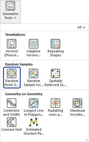
Three kinds of area of interest
- Polygons — points uniformly distributed by area; selections are honored, holes and multipart shapes respected.
- Polylines — points uniformly distributed along the lines by length.
- An integer raster with an attribute table — points uniformly distributed within the data cells; NoData is excluded, categories come from the Value field, and every output point carries its cell's Value in a Category field.
A plain extent works too, when no dataset is given. The Extent geoprocessing environment clips polygon areas when set — and for rasters it clips the read window itself, so a small analysis extent on a huge raster reads only that window. That also keeps the contiguous-region and boundary-distance options (which hold about 60 million cells in memory) available on rasters far larger than that.
The sampling design: strata and allocation
The design is set by two choices, following the stratification model of Esri's Create Spatial Sampling Locations. The sampling method defines the strata:
- No stratification — the whole area is one stratum.
- Each individual polygon or polyline is a stratum.
- Each raster category (Value field).
- Each contiguous raster region — a connected block of cells sharing one value, where connected means shared edges; two same-value regions that do not touch are different strata.
- Groups sharing a strata ID value — an integer or text field gathers polygons, polylines or raster categories into strata whose members need not be contiguous.
The sample count allocation method sets how many points each stratum receives:
- Equal count in each stratum — give the number of samples per stratum.
- Count proportional to stratum area (or length) — give the overall number, distributed by exact largest-remainder apportionment.
- Count equal to a population field — each stratum's own number; the field cannot be negative, and grouped strata sum their members.
- Count proportional to a population field — give the field and the overall number.
- By density — points per acre, square mile, hectare or square kilometer of area; per foot, mile, meter or kilometer of line length for polylines.
Density and proportional counts come from geodesic areas and lengths — true per-row cell areas for geographic rasters. Unstratified sampling offers the fixed total and density. Stratified outputs carry a Stratum field, and feature-based strata add a Src_FID link back to the source feature.
Here is the design at work, and notice where its sample count came from: the 580 in the Number-of-samples box is not a guess — it is the number the Estimate Sample Size tool recommended for this very classification (four classes, per-class proportions and precisions). The two tools are built as a pair: one computes how many samples a defensible assessment needs, the other places them. Stratified by the classified raster's categories with counts proportional to stratum area, each vegetation class receives its fair share:
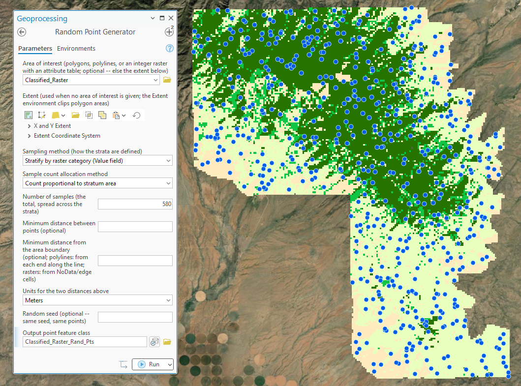
(The Kappa tutorial walks this same hand-off end to end on its own data, from sample-size estimate through stratified draw to the finished accuracy assessment.)
The two separation constraints
Both are optional, both are hard constraints, and both are given in real units (meters, kilometers, feet or miles): a minimum distance between points, and a minimum distance from the area boundary. Esri's Create Random Points offers only the first, evaluated in the dataset's own — possibly angular — units; this tool enforces the boundary separation exactly by insetting the area before sampling, so there is no buffer pre-processing step to remember. The boundary distance respects polygon outer edges and hole edges; for polylines it is measured along the line from each end (and each part's ends); for rasters it is the distance from NoData cells and the raster or read-window edge, resolved at cell precision.
Why you would want them: the boundary separation guarantees your points are isolated from influences that leak in from outside the analysis or management area. Edges are rarely representative — habitats near a boundary are often in a transition state (the familiar edge effect), and the margins of an area may be contaminated from outside: more invasive plants, or salts and pollutants drifting off roads. Pulling every sample inward by a stated distance keeps those compromised margins out of the sample. The between-point separation serves the statistics instead: samples placed close together tend to echo one another — spatial autocorrelation — so spreading them apart reduces that redundancy and helps maintain the statistical independence the downstream analyses assume (see the unit-independence discussion in About Kappa analysis for what breaking it costs).
Three ways to measure spacing along polylines
For polygon and raster areas, the minimum distance between points is what you would expect: an absolute spatial separation. Polylines offer that too, plus two smarter alternatives:
- Absolute spatial distance (the default) — no two points closer than the minimum in any direction.
- Distance measured along the polyline — only points on the same line constrain each other, by the distance you would travel along it; points on separate lines never block each other, however close they pass.
- Network distance through connected polylines — lines joined at shared endpoints and confluences (T and Y junctions, including a multipart feature's own parts) constrain each other by travel distance through the network.
Why you would want the along-the-line option: suppose you are placing survey stations along drainage-bottom polylines and require stations at least 500 meters apart, so each samples a different reach of stream. Two neighboring drainages may run parallel only 200 meters apart across a dividing ridge. With absolute spatial spacing, a station in one drainage would sterilize the adjacent reach of the neighboring drainage — blocking perfectly good stations that are kilometers away by water. Along-the-line spacing keeps the 500-meter guarantee within each drainage while letting the neighbor be sampled independently.
The network option extends the same idea to whole stream systems: a station just upstream of a fork correctly guards the first reach of both branches, while unconnected lines still never interact. The network is built over the minimum set of lines necessary — the whole feature class when unstratified, each strata-ID group's joined segments when stratifying by ID, or a single feature's own parts when stratifying by individual polyline. One caution from the plumbing: endpoints must coincide (snapped data) to count as connected, and lines that merely cross without a shared endpoint — a bridge over a stream — do not connect.
When the spacing is too tight
Random packings of circles jam near 55% coverage, well short of what orderly packing could achieve — so a request can be impossible even when the arithmetic of area and spacing looks generous. The tool checks this up front and warns, then places as many points as fit and reports the shortfall; every placed point still honors the constraints. The Advanced section controls how hard it tries: the placement-attempts-per-point budget (default 1000) is how many candidate locations each requested point may consume before the tool gives up on reaching the full count. Raise it to pack tighter at the cost of a longer run; lower it to give up faster.
Relation to Esri's sampling tools
This tool is very similar to Esri's Create Spatial Sampling Locations — the stratification and allocation choices follow the same model — except that it adds a few things: the minimum distance from the area boundary, sampling along polylines, density-based counts, real-unit distances that stay meaningful on geographic data, and a reproducibility seed. Two of that tool's output types are deliberately not duplicated here, because other Wildlife and Forestry Tools already produce them. Its Systematic (gridded) point arrays are exactly what the Repeating Shapes tool's point patterns generate, with more arrangements and full control of spacing and orientation. Its Cluster output — tessellate the study area, then keep a random subset of the tiles — is a two-tool recipe: tessellate with Repeating Shapes (hexagons, squares, triangles or rectangles), then run Select Random Records on the result, with the bonus that the subset can be sized from a confidence level and margin of error, selected in proportion to area, or made reproducible with a seed. Compared with the older Create Random Points, this tool adds the boundary distance, density counts and stratified designs. The generation is vectorized — large point sets with tight spacings place in seconds.
Geographic data and reproducibility
Geographic (latitude–longitude) data is handled in an automatic Lambert azimuthal equal-area working projection centered on the area of interest and built on the input's own datum: uniform density is exact everywhere, separation distances are true to second order at regional scales, and the output is written back in the input geographic coordinate system. The random seed makes runs exactly reproducible — the same inputs with the same seed give the same points; leave it blank for a fresh draw each run. The output inherits the boundary's coordinate system unless the Output Coordinate System environment says otherwise.
ModelBuilder
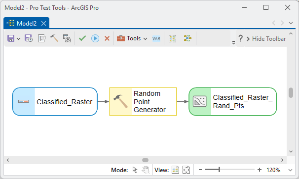
The tool's output point feature class chains directly into whatever comes next — and its sample count chains in from upstream: Estimate Sample Size's derived Recommended sample size output feeds the Number-of-samples parameter, so the statistically derived count is never retyped (the tutorial's Step 1 shows that chain):
And once your random points are on the map, remember that someone has to walk to every one of them. If you plan to hike to each point, the Estimated Shortest Path through Points tool will order them into an efficient field survey route to follow — often a substantial saving in overall effort and time.
Parameters
| Label | Explanation | Data type |
|---|---|---|
| Area of interestOptional · boundary | Polygons to fill (holes and multipart shapes handled), polylines to place points along, or an integer raster with an attribute table (NoData excluded; categories from the Value field). Selections are honored. Leave blank to use the extent parameter instead. | Feature Layer; Raster Layer |
| ExtentOptional · extent | A plain rectangular area, used when no area of interest is given. The Extent geoprocessing environment clips polygon areas when set. | Extent |
| Sampling method (how the strata are defined)Required · strata_method | No stratification; each individual polygon or polyline; each raster category; each contiguous raster region (shared edges connect); or groups sharing a strata ID value. The choices are phrased to match the input. | String |
| Strata ID fieldOptional · strata_field | The integer or text field whose values group polygons, polylines or raster categories into strata (members need not be contiguous). The ObjectID field also qualifies. For rasters this is an attribute-table field. | Field |
| Sample count allocation methodRequired · alloc_method | How many points each stratum receives: an equal count, a count proportional to stratum area (or length), a count equal to or proportional to a population field, or a density. Unstratified sampling offers the fixed total and density. | String |
| Number of samplesOptional · n_points | The overall number of samples, distributed across the strata (proportional methods) or the whole area in proportion to area or length. | Long |
| Number of samples per stratumOptional · n_per_stratum | The number of samples each stratum receives (equal-count allocation). | Long |
| Population fieldOptional · population_field | A non-negative numeric field driving the equal-to or proportional-to population allocations: per polygon or polyline (a grouped stratum sums its members), or a raster attribute-table field per category. | Field |
| Density: points per unitOptional · density | How many points per unit — e.g. 0.5 points per hectare, or per mile of line for polylines, or per hectare of each category for rasters. Counts come from geodesic areas and lengths. | Double |
| Density unitOptional · density_units | Acre, Square Mile, Hectare or Square Kilometer for areas; Foot, Mile, Meter or Kilometer of line length for polylines. | String |
| Minimum distance between pointsOptional · min_spacing | No two points will fall closer together than this (a hard constraint). If the count cannot be met at this spacing the tool warns and places as many as fit. | Double |
| How the minimum distance is measuredOptional · spacing_type | Polylines only: absolute spatial distance (default); distance measured along the polyline (only points on the same line constrain each other); or network distance through connected polylines (travel distance through shared endpoints and confluences). | String |
| Minimum distance from the area boundaryOptional · boundary_gap | No point will fall closer to the area's boundary than this — polygon outer edges and hole edges; for polylines, measured along the line from each end; for rasters, the distance from NoData/edge cells. | Double |
| Units for the two distances aboveOptional · linear_units | Meters, Kilometers, Feet or Miles. | String |
| Random seedOptional · random_seed | The same seed with the same inputs reproduces the same points exactly. Leave blank for a fresh draw each run. | Long |
| Placement attempts per pointOptional · max_attempts | Advanced: how many candidate placements each point may consume before the tool gives up on reaching the full count (used when a minimum spacing is set; default 1000). Raise it to push harder in tightly packed areas; lower it for a faster give-up. | Long |
| Output point feature classRequired · out_fc | The output points, with Point_ID; stratified runs add a Stratum field, feature-based strata add Src_FID, and raster runs add the cell's Category. | Feature Class |
Python
Half a point per hectare within each polygon, at least 100 m apart and 50 m inside the boundary, reproducible with a seed (the comment block lists every method string — matching is by prefix):
import arcpy
arcpy.ImportToolbox(r"C:\path\to\JennessEnterprisesTools.pyt")  # your install path
# strata_method options (matching is by prefix):
#   "No stratification (the whole area is one stratum)"
#   "Stratify by individual polygon" / "... polyline"
#   "Stratify by raster category (Value field)"
#   "Stratify by contiguous raster region"
#   "Stratify by strata ID field"  (+ strata_field)
# alloc_method options:
#   "Fixed total number of points"  (unstratified)
#   "Equal count in each stratum"  (+ n_per_stratum)
#   "Count proportional to stratum area"  (+ n_points)
#   "Count equal to a population field"  (+ population_field)
#   "Count proportional to a population field"
#   "By density (points per area unit)" / "... length unit"
# density_units: "Acre" / "Square Mile" / "Hectare" / "Square Kilometer"
#   (for polylines: "Foot" / "Mile" / "Meter" / "Kilometer")
# linear_units: "Meters" / "Kilometers" / "Feet" / "Miles"
arcpy.jenness.RandomPointGenerator(
    boundary=r"D:\data\study.gdb\subplots",
    strata_method="Stratify by individual polygon",
    alloc_method="By density (points per area unit)",
    density=0.5, density_units="Hectare",
    min_spacing=100.0, boundary_gap=50.0,
    linear_units="Meters", random_seed=42,
    out_fc=r"D:\data\study.gdb\sample_points")
Recommended citation
Credits
By Jeff Jenness, Jenness Enterprises (www.jennessent.com). A modernized port of the author's ArcView 3.x Random Point Generator (randpts.avx) extension.
Licensing information
Works at every ArcGIS Pro license level (Basic, Standard, Advanced). No extension licenses are required.
Related tools and pages
- Estimate Sample Size — how many samples the design needs; its derived count feeds this tool in ModelBuilder.
- Select Random Records — random selection from features that already exist, including the tessellate-then-subset cluster recipe.
- Repeating Shapes — systematic (gridded) point arrays and tessellations, complementing this tool's random designs.
- Random Sample Array Generator — random placement of whole sampling arrays (grids, transects, circles), built on this tool's chassis.
- Classification Accuracy (Kappa) — the assessment a stratified design feeds.
- Kappa analysis tutorial — this tool drawing a real stratified design (Step 2).
- Estimated Shortest Path through Points — order the points into an efficient field survey route for hiking to every one.