

Kappa Analysis Tutorial
Kappa_Tutorial_Data.gdb): a
supervised vegetation classification (as a raster and as polygons)
and 362 field samples surveyed independently by two observers.
Download the tutorial data
here (0.3 MB) — unzip it anywhere convenient, add
the geodatabase's datasets to an ArcGIS Pro map, and you can
follow along click for click.
This tutorial follows one complete accuracy assessment from start to finish: planning the sample size, drawing the sampling design, running the assessment once per field observer, reading each block of the report, comparing the two analyses — first by hand with the Compare Accuracy Analyses tool, then automatically in a single run — and confirming the results independently in R. The steps form a natural workflow — but you are not chained to it. Every tool accepts generic inputs, so you can enter anywhere: bring your own samples, type a matrix's worth of values, or compare kappas straight from the literature.
The data
The tutorial geodatabase holds five datasets. The classification is
a supervised vegetation classification of a portion of the
Pinaleños Mountains, Arizona, with four classes: Mixed Conifer
forest (35.7% of the classified area), Oak/Juniper woodland (43.0%), Bare
Ground/Grass (13.2%) and Pine/Oak woodland (8.1%). It comes in two
interchangeable forms — Classified_Raster, whose
attribute table carries the class names in a field named
S_VALUE, and Classified_Polygons, the same
classification as polygons with the names in VEG_LABEL
— so you can run the assessment against whichever form your own
projects use.
The field samples are 362 surveyed locations, each visited
independently by two observers who recorded the vegetation class they
found in a field named COARS_VEG. They appear three ways:
Observer_1 and Observer_2 hold each survey
separately, and Observers_1_and_2 stacks both surveys in
one feature class (724 points) with an Observer field
telling them apart — the shortcut dataset for Step 8. (Why
the samples were collected the way they were is a story for
Step 1.)
Step 1 — How many samples would we need?
In a perfect world, we would start the research by generating random sample locations across the landscape. The randomness allows us to apply the knowledge we gain to the larger ecological system, rather than settling for a single-shot analysis that only tells us about our sample points. Ideally we would be able to reach and survey all our sample points, and we would save costs and resources by sampling only the minimum number necessary to achieve the confidence level we want from our statistics.
In this perfect world, we would use our Estimate Sample Size tool to size our sampling array before we began our field surveys. For example, suppose we had initially classified our landscape into 4 important categories, and we therefore have an estimate of the proportion of the landscape that lies in each category. Suppose also that we want our field survey effort to tell us the classification accuracy with 95% confidence and a 10% level of precision — meaning that we are willing to accept an accuracy estimate that lands within 10 percentage points of the true accuracy, and we want a survey design that would deliver an estimate that close in 95 out of every 100 repetitions. Given these initial conditions, we can use the Estimate Sample Size tool to tell us the number of sample points necessary, given that we know the proportion covered by the largest category (Oak/Juniper, at 43%):
| Class | Hectares | Proportion |
|---|---|---|
| Oak/Juniper | 18,321 | 43.0% |
| Mixed Conifer | 15,224 | 35.7% |
| Bare Ground/Grass | 5,606 | 13.2% |
| Pine/Oak | 3,466 | 8.1% |
| Total | 42,616 | 100% |
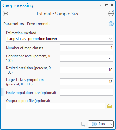
Based on this, we see that we would need 153 randomly-distributed points (and stratified within categories, so that 43% of the random points fall within that Oak/Juniper category). You can find this value in the Tool Results window:
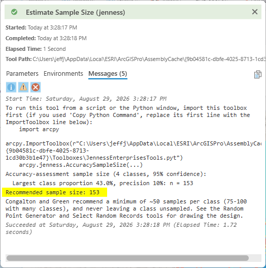
Refer to the Estimate Sample Size online help page for details on how this tool can be run given different analytical goals. If we knew nothing about the relative proportions covered by the landscape categories, for example, we would need 156 randomly-distributed points. And if our goal were not to estimate our classification accuracy, but rather to estimate the true areas covered by each category on the landscape, then we would set up the Estimate Sample Size tool to target a standard error of overall accuracy (the Olofsson et al. 2014 method): pinning overall accuracy to within ±1 percentage point of standard error takes roughly 774 points if we are optimistic about our conjectured user's accuracies (85–95%), and over 2,200 points if we guess pessimistically near 50%. That is an honest planning lesson worth absorbing: inaccurate classifications need far more samples to pin down.
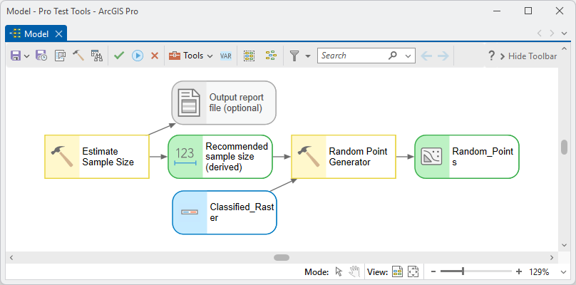
In the real world, when we originally did this analysis, we were limited by rough topography and simply unable to survey randomly, and consequently we applied a systematic approach by sampling at regular intervals along navigable trails. We knew our study design was weakened by this lack of randomness, so we sampled more points than we would have originally estimated to be necessary. Our 362 samples comfortably exceeded the multinomial requirements and give about 90 samples per class on average — well above Congalton and Green's 50-per-class rule of thumb. Had we needed to draw the design, the Random Point Generator (stratified by the classification's categories) or Select Random Records would be the next stop, and the recommended sample size flows into them directly in ModelBuilder:
Step 2 — Drawing the design with the Random Point Generator
We did not actually generate random points for this study — the topography vetoed that, as it may for yours. But in the interests of showing the complete analytical flow path, here is how we would draw the 153 random points, stratified by the proportion of the landscape in each category.
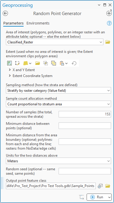
Open the Random Point Generator (Geometric Tools group). In the tool window:
- Set the Area of interest to
Classified_Raster. An integer raster with an attribute table works directly as a stratification source. - Set the Sampling method to Stratify by raster category (Value field), so each of the four vegetation classes becomes its own stratum.
- Set the Sample count allocation method to Count proportional to stratum area, so that the 43% Oak/Juniper category receives 43% of the points.
- Set the Number of samples to 153 — the number Step 1 recommended.
- Pick a name and location for the Output point feature
class. I recommend saving it to your project geodatabase and
naming it
Sample_Points.
The filled dialog should look something like the following:
And the result is the sampling distribution we would have wished for — 153 random points, spread so that each vegetation category receives its proportional share:
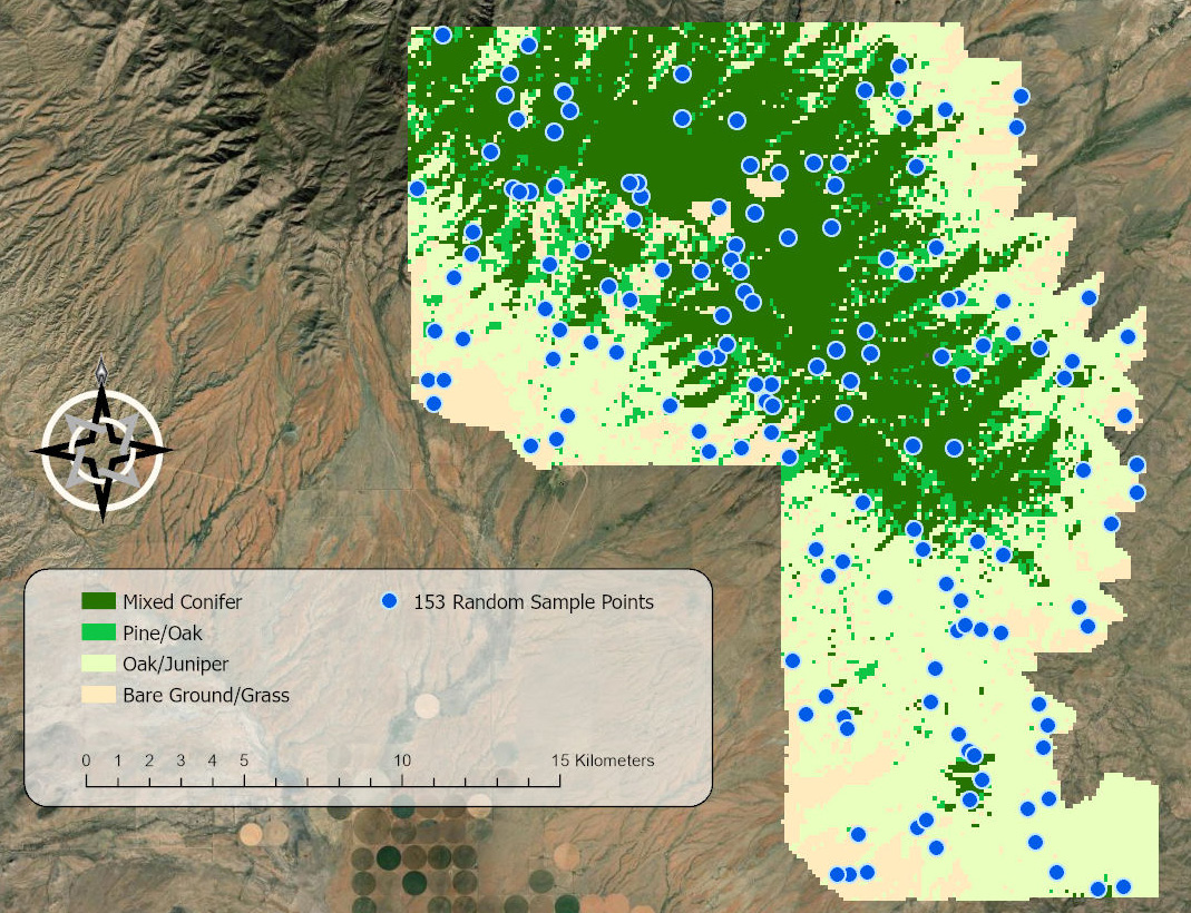
The tool has considerably more depth than we needed here — minimum spacing between points, boundary offsets, other stratification and allocation recipes — all covered on the Random Point Generator help page.
Step 3 — Go get the data
Probably the most fun part of the whole analysis, for most of us: actually going out and surveying the sample points. Time to go get the data. There is no dialog to fill in for this step and no button to click — just boots, datasheets and a GPS unit. For this study it meant working through some genuinely rugged Pinaleños country, twice over (once per observer), recording the vegetation class actually found at each of 362 locations. We will not pretend that is a small investment of time and effort — it is usually the largest line in the whole project budget. But let's be honest with ourselves: days in the field like these are why most of us went into ecological analysis in the first place. The statistics in the steps that follow are simply how we make sure all that boot leather ends up telling us something durable about the landscape.
For the tools downstream, the field protocol reduces to one
essential: at each sample point, record the class you actually find
in a field of its own (ours is COARS_VEG) —
independently of what the classification claims. Everything else you care to
record while you are standing there is a bonus.
Step 4 — Running the assessment on Observer 1
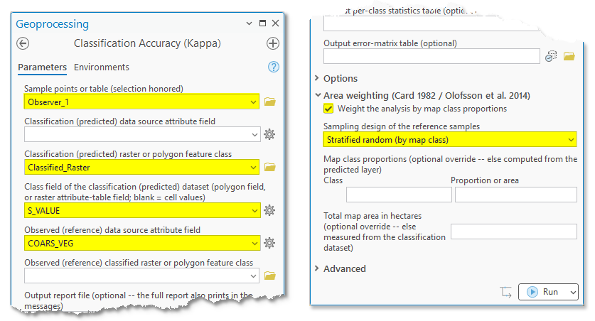
Back at the computer: remember that our actual samples are not the random points of Step 2 but the 362 systematically-surveyed locations, and the first survey to assess is Observer 1's. Open Classification Accuracy (Kappa) (Ecological Analysis group). In the tool window:
- Set the Sample points or table to
Observer_1. - Set the Classification (predicted) raster or polygon feature
class to
Classified_Raster. - Set the Class field of the classification dataset to
S_VALUE. This is the raster attribute-table field holding the class names, so the extracted classes match the reference field's vocabulary — names compared to names, not names to cell codes. - Set the Observed (reference) data source attribute field
to
COARS_VEG— the class each observer actually found on the ground. Note that in this example the observed values live in the sample point feature class itself, as an attribute of the points — likely the more common scenario, since field crews usually record what they find directly on the sample records. If your reference classes live elsewhere, specify a raster or polygon feature class in the boxes below instead. - Check Weight the analysis by map class proportions. This adds the Card/Olofsson area-weighted block; the class proportions and the total classified area are measured from the raster automatically.
- Leave the Sampling design of the reference samples at Stratified random (by map class), the default — the variance formulas differ between designs (Card 1982).
The filled dialog should look something like the following (the dialog is tall, so it is shown here in two pieces — the top half on the left, the lower half on the right):
Step 5 — Reading the report
The tool prints the full report in the messages (and to a text file if you asked for one). Walking through Observer 1's blocks in order:
The error matrix
| Observed (reference) | ||||||
|---|---|---|---|---|---|---|
| Bare Ground/ Grass | Mixed Conifer | Oak/ Juniper | Pine/Oak | Total | ||
| Predicted (classification) |
Bare Ground/Grass | 16 | 3 | 12 | 3 | 34 |
| Mixed Conifer | 8 | 115 | 25 | 26 | 174 | |
| Oak/Juniper | 22 | 7 | 79 | 11 | 119 | |
| Pine/Oak | 1 | 5 | 17 | 12 | 35 | |
| Total | 47 | 130 | 133 | 52 | 362 | |
Read the off-diagonal cells before any statistic, because they tell several different stories at once. The largest single error cell is 26: samples where the crew stood in Pine/Oak but the classification said Mixed Conifer. Only 52 Pine/Oak samples were observed in total, so that one cell has already swallowed half the class — the main reason Pine/Oak's producer's accuracy will look so poor below. Summing each pair of classes in both directions tells another story: Oak/Juniper and Bare Ground/Grass trade 34 samples between them (12 misclassified in one direction, 22 in the other), the largest two-way confusion on the matrix. And Oak/Juniper trades 32 with Mixed Conifer (25 + 7), which is worth a pause, because those two types generally do not even neighbor each other on the mountain: the vegetation follows the elevation gradient, with Oak/Juniper at the lower elevations, Pine/Oak in the middle and Mixed Conifer up high (Bare Ground/Grass can appear anywhere), so the classification is confusing classes from opposite ends of the gradient, not blurring a shared boundary. Three observations from one table, and not one of them visible in any overall statistic.
Overall statistics
- Overall accuracy 0.6133 (222 of 362), with exact binomial 95% CI 0.5609 to 0.6637 — the plain proportion correct.
- No-information rate 0.3674, P < 0.00001: always guessing the commonest class would score 37%, and the classification is convincingly better than that.
- McNemar–Bowker marginal-symmetry test: chi-square 31.85 on 6 df, P = 0.00002. This one asks whether the classification's mistakes are an even trade — whether about as many samples get misclassified from class A into class B as from B into A. Here they emphatically are not: look at the matrix margins, where the classification claims 174 samples' worth of Mixed Conifer against the 130 the observer found, while shorting Pine/Oak (35 predicted, 52 observed). A P value this small says that directional bias is real, not sampling luck — the classification systematically over-draws some classes at the expense of others. This is an early warning that the raw class acreages are biased, and it is exactly the problem the error-adjusted area estimates at the end of the report will correct.
- Cohen's Kappa 0.4317 (variance 0.001184, Z = 12.5, 95% CI 0.364 to 0.499): agreement is 43% better than chance. Note the Kappa interval and the accuracy interval answer different questions — the first about chance-corrected agreement, the second about the proportion correct — and the report carries both.
- Gwet's AC1 0.5009: read it exactly like Kappa — agreement beyond chance, on the same scale — but built on a chance model that stays stable when one class dominates the landscape. When the two disagree sharply, prevalence is distorting Kappa; here they sit reasonably close (0.43 and 0.50), so Kappa's story can be taken at face value.
- Pontius–Millones disagreement: quantity 0.12, allocation 0.27 — most of this classification's error is in where classes were put, not in how much of each it drew.
Per-class statistics
The per-class table is where management decisions live, so let's not rush past it. The key columns for Observer 1:
| Class | n predicted | n observed | User's accuracy | Producer's accuracy |
F1 | Balanced accuracy |
|---|---|---|---|---|---|---|
| Bare Ground/Grass | 34 | 47 | 0.4706 | 0.3404 | 0.3951 | 0.6416 |
| Mixed Conifer | 174 | 130 | 0.6609 | 0.8846 | 0.7566 | 0.8152 |
| Oak/Juniper | 119 | 133 | 0.6639 | 0.5940 | 0.6270 | 0.7097 |
| Pine/Oak | 35 | 52 | 0.3429 | 0.2308 | 0.2759 | 0.5783 |
Take one row and read it end to end. Pine/Oak was predicted at 35 samples but observed at 52, and its diagonal cell in the error matrix holds 12. User's accuracy reads the classification's own claims: of the 35 samples it calls Pine/Oak, 12 really are — 12/35 = 0.3429, so a manager standing on ground classified as Pine/Oak has roughly a one-in-three chance of actually being in it. Producer's accuracy reads the ground: of the 52 Pine/Oak stands the observer found, the classification caught 12 — 12/52 = 0.2308, so more than three-quarters of the real Pine/Oak is missing from the classified dataset. If Pine/Oak matters to your study species, this single row matters more than any overall statistic on the page.
Now contrast Mixed Conifer, where the two accuracies split in the opposite way: producer's accuracy is excellent (115/130 = 0.8846 — when you are standing in Mixed Conifer, the classification almost always knows it) while user's accuracy is mediocre (115/174 = 0.6609 — a third of what it calls Mixed Conifer is really something else, much of it that missing Pine/Oak). Reading the two accuracies as a pair tells you not just how good a class is, but which direction it fails in: Mixed Conifer is over-claimed, Pine/Oak is swallowed.
The remaining columns condense that pair into single scores. F1 is the harmonic mean of user's and producer's accuracy — a class only scores well if both are good, and the harmonic mean punishes imbalance (Mixed Conifer's 0.88/0.66 pair earns 0.76, not the 0.77 a plain average would give; weaker pairs are punished harder). Balanced accuracy averages how well the class's members are found (sensitivity, which is producer's accuracy by another name) with how well non-members are excluded (specificity); 0.5 is coin-flip performance, so Pine/Oak's 0.5783 sits uncomfortably close to guessing.
Below the table the report prints two summary lines that are easy to skim past but worth understanding:
- Macro-F1 (0.5136) is the plain average of the four per-class F1 scores — every class counts equally, no matter how small its share of the landscape. Compare it against overall accuracy (0.6133), which lets the big classes dominate: the gap between the two numbers says the small classes are faring worse than the headline figure suggests. When the two are close, quality is even across classes.
- Weighted averages (sensitivity 0.6133, specificity 0.8711, omission 0.3867, commission 0.1289) re-average the per-class numbers with each class weighted by its share of the observed samples. Weighted sensitivity works out to exactly the overall accuracy — a reassuring internal consistency, not a coincidence — and the omission and commission figures are the complements of the sensitivity and specificity beside them: the sample-weighted rate at which class members were missed, and at which samples were falsely drafted into classes they do not belong to.
Area-weighted estimates and error-adjusted areas
Because the analysis was weighted by the class proportions, the report finishes with the Olofsson block. The tool measured the total classified area automatically — 42,615.8 ha of analyzed classes — and corrected each class's acreage for the misclassification the matrix revealed:
| Class | Classification says | Error-adjusted estimate |
|---|---|---|
| Bare Ground/Grass | 13.2% (5,606 ha) | 16.0% ± 2.0% (6,824 ± 857 ha, or 5,967 to 7,681 ha) |
| Mixed Conifer | 35.7% (15,224 ha) | 28.5% ± 1.8% (12,129 ± 760 ha, or 11,369 to 12,889 ha) |
| Oak/Juniper | 43.0% (18,321 ha) | 42.3% ± 2.5% (18,012 ± 1,051 ha, or 16,961 to 19,063 ha) |
| Pine/Oak | 8.1% (3,466 ha) | 13.3% ± 1.8% (5,651 ± 752 ha, or 4,899 to 6,403 ha) |
This is the block worth pausing over. The classification under-represents Pine/Oak by roughly forty percent of its true extent — real Pine/Oak is being absorbed into the Mixed Conifer class — while Mixed Conifer is over-claimed by about a fifth. Kappa told us agreement was moderate; the area estimates tell us specifically which hectares to distrust, with error bars suitable for a manuscript.
Step 6 — The second observer
Run the tool a second time with Sample points or table set to
Observer_2 and every other entry unchanged. The report has
the same structure; the headline numbers land close to
Observer 1's:
| Observer 1 | Observer 2 | |
|---|---|---|
| Overall accuracy | 0.6133 (222 of 362) | 0.5994 (217 of 362) |
| Cohen's Kappa | 0.4317 | 0.4131 |
| Kappa variance | 0.001184 | 0.001134 |
| Gwet's AC1 | 0.5009 | 0.4825 |
The same story holds class by class — Mixed Conifer strong from the producer's side, Pine/Oak weak from both — which is itself informative: the failings look like properties of the classified dataset, not of whoever did the surveys.
Step 7 — Comparing the analyses
Are the two observers statistically distinguishable? Open Compare Accuracy Analyses and type one row per analysis into the value table, straight from the two reports: Observer 1 with kappa 0.4317 and variance 0.001184, Observer 2 with kappa 0.4131 and variance 0.001134. The tool prints:
- Each kappa's own Z test against chance (both P < 0.00001 — both analyses beat guessing).
- Pairwise test: Z = 0.386, P = 0.700 — no evidence the observers differ.
- Common Kappa (Fleiss 1981¶): 0.4222, chi-square 0.149 on 1 df, P(equal) = 0.700 — the two analyses can be summarized by one pooled kappa.
The filled tool and its results should look something like the following:
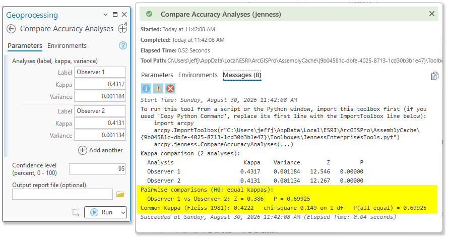
The two observers are statistically indistinguishable — a reassuring result, and precisely the multiple-interpreter agreement question that even Kappa's critics agree the statistic answers well (see the Kappa debate). Notice what this tool asked for: just a kappa and a variance per analysis. Nothing requires the analyses to share sample points, sample sizes, software, or even a decade — two crews surveying entirely different plots compare just as naturally, and you can test your model against a kappa published in the literature by typing two rows.
One honest nuance runs the other way. The Z and common-kappa tests assume the analyses are independent samples — which different plots satisfy exactly. Our two observers stood at the same 362 points, so their kappas are positively correlated and the test runs slightly conservative: real differences must be a little larger than usual to register. A significant result can therefore be trusted; a borderline non-significant one deserves a second look with McNemar's paired test (Foody 2004)¶, the sharp tool for same-sample comparisons. Here, at P = 0.700, the observers agree by either reading.
Step 8 — The one-run shortcut
Because both surveys live in one feature class, we could have done
Steps 4 through 7 in a single run — the samples need not share
locations, only a table and a field that tells the analyses apart.
Point the tool at Observers_1_and_2 and set the
Analysis field (under Options) to
Observer. The tool splits the samples
by that field's values, produces one complete report block per observer
(identical, number for number, to the separate runs above), and
finishes with the same comparison block: Z = 0.386,
P = 0.700, common kappa 0.4222. The filled dialog (tall, so
shown in three pieces) and the tail of its results:
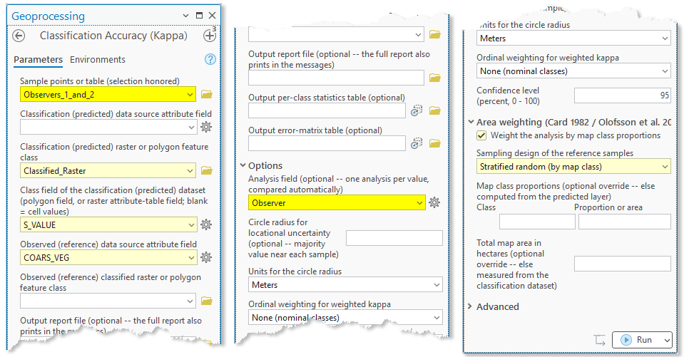
Observers_1_and_2 and the
Analysis field (under Options) is set to
Observer.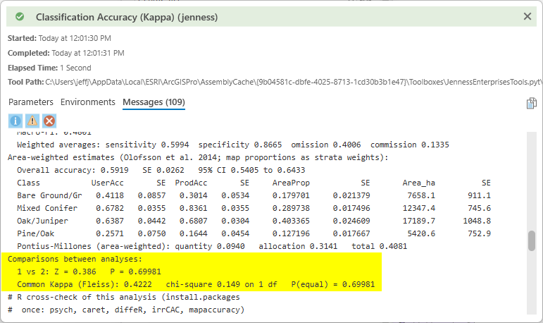
Use whichever form fits your bookkeeping. Separate runs keep each model or observer in its own dataset and report — and Compare Accuracy Analyses will reconcile them later, even from typed values. The analysis field suits samples that already live in one table: per observer, per model, per imagery date — one run, comparisons included, and a single R snippet that reproduces everything.
Step 9 — Confirming the results in R
Every report ends with a ready-to-run R snippet carrying your own
error matrix and strata weights. Paste it into R and it reproduces the
analysis with the reference packages — psych for
Kappa and its variance, caret for the per-class suite,
diffeR for the Pontius disagreements, irrCAC
for AC1, and mapaccuracy for the Olofsson areas. Those
five packages are the only setup R needs, installed once:
install.packages(c("psych", "caret", "diffeR", "irrCAC", "mapaccuracy"))With an analysis field, the snippet carries every observer's matrix and finishes with the same pairwise Z and common-Kappa tests. Running it for this dataset confirms each number above to the printed digit — we encourage the skeptical reader to try; skepticism is, after all, what this whole analysis is for.
Where to go from here
- Join the per-class statistics table back to your classified layer to symbolize per-class accuracy spatially.
- Run competing classifications through the same samples with the analysis field — or as separate runs fed to Compare Accuracy Analyses — and let the comparison block pick your model; fall back on multi-criteria selection when significance is out of reach (see the Mexican Jay case study in About Kappa analysis).
- In ModelBuilder, the workflow chains in two pieces with a field season in between — no model can wire all four tools together, because Step 3 happens outdoors. Before the field work: Estimate Sample Size → Random Point Generator, with the derived recommended sample size feeding the point count (the model pictured in Step 1). After you have been out and gotten some sun: Classification Accuracy → Compare Accuracy Analyses, with the derived kappa and variance flowing between them — or skip the second chain entirely by merging the surveys into one feature class and letting the analysis field run the comparison in a single tool.