

Select Random Records
Summary
The surest way to pick a subset that stands for the whole is to let chance pick it. When every record has the same chance of being chosen, nothing about a record, not its size, its location, its value or how easy it is to get to, can make it more likely to be in the sample than any other. The sample cannot lean toward the convenient or the conspicuous, because no one chose it. A subset picked by eye, or chosen because a site is easier or quicker to get to, has a bias even when the person picking it doesn't want it to. And because a random sample differs from the population only by chance, the size of that difference can be worked out, which is what lets a result from the sample be reported with a confidence level and a margin of error.
This tool selects a random or systematic sample of the features in a layer, or of the rows in a table. The sample can be a fixed number of records, a percentage, a size worked out from a confidence level and a margin of error, a number selected with the larger features more likely to be chosen, or a systematic sample of every Xth record. The result is an ordinary selection on the layer or table, so whatever you would do with a selection, you can now do with a sample: copy it out, calculate a field on it, summarize it, or hand it to a field crew.
The tool offers the four standard ways of combining a new selection with an existing one, and each of them changes which records the sample is selected from. The sample can also be restricted to an analysis extent or to the inside of a polygon boundary, and a random seed makes any random selection exactly repeatable.
Usage
The tool applies a selection to the input. Nothing is copied and no new dataset is made. See Keeping the sample for how to turn the selection into a dataset of its own.
The input has to be a layer or a table view, which in practice means a feature layer or a standalone table in a map. A dataset on disk has nowhere to show a selection, so the tool warns about one in the dialog and stops if it is run on one. A definition query on the layer is always honored: the sample is selected only from the records the layer shows.
Seven ways to choose the sample
| Sampling method | What is selected |
|---|---|
| Fixed number of records | The number you give, selected at random with every record equally likely. If you ask for more records than there are, the tool says so and selects them all. |
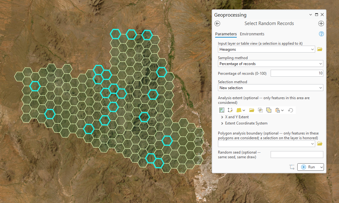
| Percentage of records | That percentage of the records, rounded to the nearest whole record and never fewer than one. |
| Sample size calculated from a confidence level and margin of error | The number of records needed to estimate a proportion to a stated precision. See A calculated sample size. |
| Fixed number, probability proportional to area / length | The number you give, selected so that larger polygons or longer lines are more likely to be chosen. See Proportional to area or length. |
| Systematic: every Xth record | Every Xth record in the order of a field you choose. See Systematic selection. |
| Systematic: odd-numbered records Systematic: even-numbered records |
Every other record in that order: the 1st, 3rd, 5th and so on, or the 2nd, 4th, 6th and so on. |
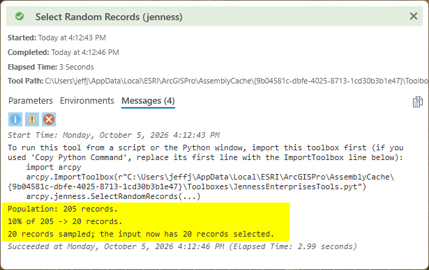
The first four select at random, and the same record is never chosen twice. Whichever method is used, the messages report the size of the population the sample was selected from, how the sample size was arrived at, and how many records are selected when the tool has finished.
A calculated sample size
With this method you do not say how many records you want. You say how good an answer you need, with two numbers, and the tool works out how many records that takes. An example shows what the two numbers mean and what the sample is good for.
A season of camera trapping has produced 12,000 photographs, and software has tagged each one with the species it shows. The tags have to be checked, but checking a photograph by eye takes a minute, and checking all 12,000 would take weeks. The question is: how many photographs do I have to check to be able to say what share of all 12,000 are tagged correctly?
That depends on how precise an answer you need, and the two numbers say so:
- The margin of error is how far the sample's answer may be from the truth. A margin of 5 means that if the photographs you check are 91% correct, the share of all 12,000 that are correct is within 5 percentage points of that, somewhere between 86% and 96%.
- The confidence level is how much that range can be trusted. At 95%, if you selected sample after sample this way, 95 of every 100 such ranges would contain the true share.
At 95% confidence and a 5% margin, the tool works out that 373 photographs are enough, and selects them. You check the 373 and find 340 tagged correctly, which is 91%. You can now report that between 86% and 96% of the whole season's photographs are tagged correctly, with 95% confidence, having looked at 3% of them. The sample is sized for the worst case, a share near 50%, so for a share as lopsided as 91% the range is in fact tighter, about 88% to 94%.
The same sample answers any other yes-or-no question about the photographs to the same precision: the share taken at night, the share with more than one animal in the frame, the share the software left untagged. Any proportion counted among the 373 holds for the 12,000 within 5 points, with the same 95% confidence.
The question has the same shape whenever a dataset is too large to check record by record: what share of a county's parcels carry a wrong land-use code, what share of 40,000 address points sit on the wrong side of the street, what share of a vegetation map's polygons are labeled right. Auto Calculate sizes the check, selects the records, and the share found among them stands for the whole.
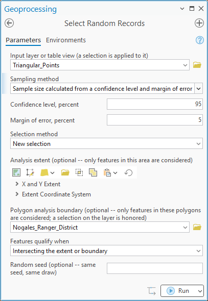
The same method on the map. We have a regular grid of sample points laid over southern Arizona, and we want to sample the ones that fall in the Nogales Ranger District, to find out at what share of them an invasive grass has taken hold. We want to be 95% confident of the answer, with a 5% margin of error. The district is a polygon layer, so it goes in as the polygon analysis boundary, and a point qualifies by intersecting it:
The tool finds 142 points in the district, works out that 104 of them have to be visited, and selects them:
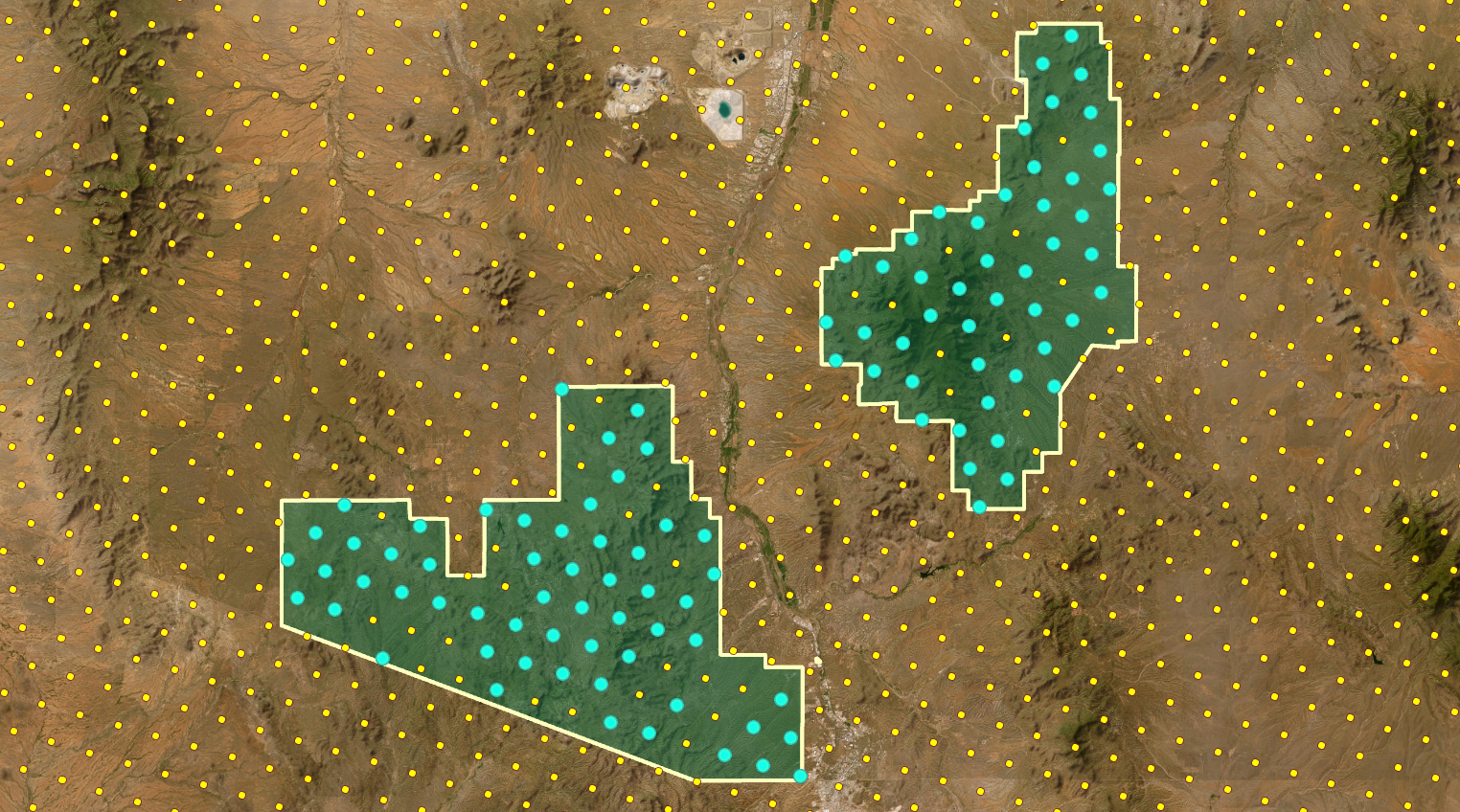
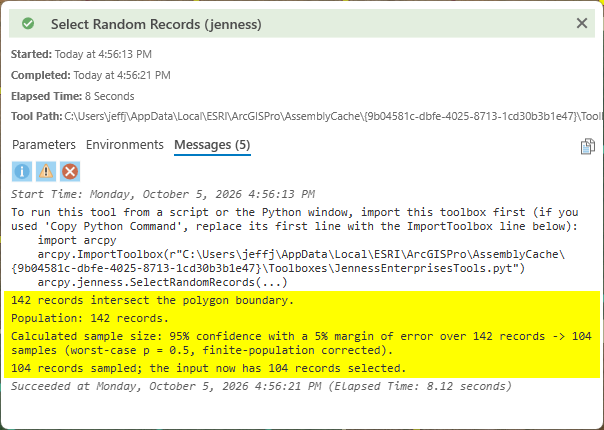
Why so many? 104 of 142 is nearly three quarters of the points, where the camera-trap example got by with 3% of its photographs. The reason is that the precision of a sample comes from the number of records in it, and not from the share of the population they make up. Pinning a proportion down to within 5 points at 95% confidence takes about 385 observations when the population is large, and 385 observations say as much about a population of a million as about one of ten thousand. A population of 142 cannot supply 385. Here the correction for the size of the population does its work: with so few points to begin with, every point checked settles a real share of the whole, and 104 are enough. But 104 is still most of them. The smaller the population, the larger the share of it that has to be examined. At 95% confidence and a 5% margin:
| Records in the population | 20 | 50 | 100 | 142 | 200 | 500 | 1,000 | 10,000 | 1,000,000 |
|---|---|---|---|---|---|---|---|---|---|
| Records to sample | 20 | 45 | 80 | 104 | 132 | 218 | 278 | 370 | 384 |
| Share of the population | 100% | 90% | 80% | 73% | 66% | 44% | 28% | 4% | 0.04% |
So a small population is the one case in which this method can disappoint. It never fails: when the population is tiny, the calculated sample is simply all of it, and the tool selects every record and says so in its messages. At 95% and 5% that is what happens for twenty records or fewer, and there is then nothing to be gained by sampling at all. With a few hundred records the method still asks for most of them. It comes into its own when the population runs to thousands, where a few hundred records stand for all the rest.
When the population is small and the field work is dear, the honest remedies are a wider margin or a lower confidence, and the margin is the stronger lever. For the 142 points, a 10-point margin at 95% confidence brings the sample down to 58, where dropping to 90% confidence at a 5-point margin only brings it to 94.
Behind the two numbers is this calculation. The sample size is:
where z is the standard normal value for the two-sided confidence level (1.96 for 95%), m is the margin of error as a fraction, and p is the proportion being estimated. The tool sets p to 0.5, which is the value that calls for the largest sample, so the answer is safe whatever the true proportion turns out to be. The result is then corrected for the size of the population, N, and rounded up:
This is the calculation Esri gives for the Auto Calculate option of its Select Random Sample tool, and the correction for the population is the same finite population correction that Estimate Sample Size uses, written another way.
You can bring down the sample size quickly if you are willing to accept a larger margin of error. If you accept a margin of error twice the size, you bring down the necessary sample size roughly 4 times. For a very large population at 95% confidence:
| Margin of error | 10% | 5% | 3% | 2% | 1% |
|---|---|---|---|---|---|
| Records to sample | 97 | 385 | 1,068 | 2,401 | 9,604 |
The confidence level matters less. At a 5% margin, the same very large population needs 271 records for 90% confidence, 385 for 95% and 664 for 99%.
This method sizes a sample for a single yes-or-no proportion: the share of the records that have some property. Each record is a yes or a no, so the count of yeses in the sample is a binomial quantity, and the formula is the normal approximation to the binomial. The property can be any question with a yes or no answer for each record, and it need not be a yes-or-no field. Is the mapped class correct here? Is this spring above 1,500 m? Is it a cave spring? Each of those is a proportion, and one sample sized this way answers all of them.
What the method does not size a sample for is a quantity that is measured rather than counted, such as the mean elevation of the springs. That is a standard calculation too, and it rests on the standard error of the mean. The margin of error is z times the standard error, and solving that for the sample size gives:
Here m is the margin of error in the units of the measurement, meters of elevation for the springs, and σ is the standard deviation of the measurement: how much the elevations vary from spring to spring. That is the catch. The standard deviation has to be known, or guessed, before the sample is selected. A small pilot sample will give it, and Attribute Summary Reports reports the standard deviation of a numeric field. An earlier study may give it. Failing both, a quarter of the range of the values is a rough stand-in. This tool does not make the calculation, but once you have the number, Fixed number of records selects the sample. Lesson 2 of Penn State's online course STAT 506, Sampling Theory and Methods, works through the calculation with examples, and also derives the formula for a proportion that this tool uses.
An assessment of a classification with several classes also asks more of the sample, and Estimate Sample Size is the tool for that.
Proportional to area or length
In an ordinary random sample every record has the same chance, so a sliver polygon is as likely to be chosen as one that covers a mountain range. That is right when the records themselves are what is being studied. It is wrong when the ground is what is being studied, because most of the sample then lands on whatever kind of feature is most numerous and not on what covers the most land.
With Fixed number, probability proportional to area / length, the chance of a feature being chosen follows its size: geodesic area for polygons, geodesic length for polylines. A polygon twice the size of another is twice as likely to be selected. For a single selection, the effect is the same as dropping a pin at random on the map and taking the polygon it lands in. This is known as probability proportional to size sampling. The method needs polygons or polylines, and the dialog turns it away for points and tables.
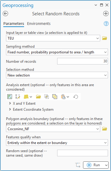
An example. We have the Terrestrial Ecological Units (TEU) of the Region 3 forests, which vary a great deal in size, and we want to select 30 of them in the Coconino National Forest. So the Coconino goes in as the polygon analysis boundary, with only the polygons that lie entirely within it considered. We run the tool twice, and the only thing we change is the sampling method:
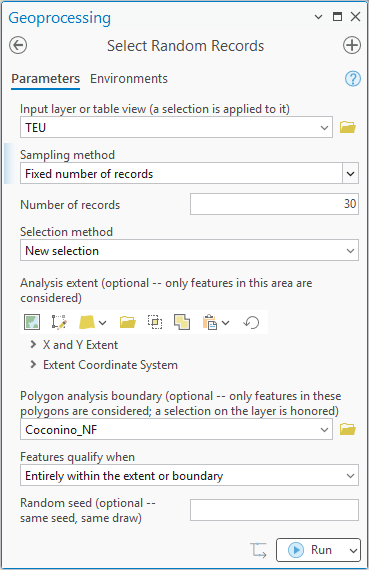
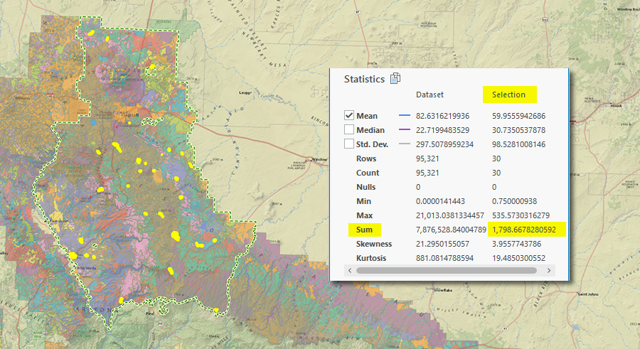
With Fixed number of records, every polygon has the same chance, and we get 30 polygons that cover 1,799 hectares between them:
With Fixed number, probability proportional to area / length, we again get 30 polygons, but this time they cover 47,954 hectares, about 27 times as much ground:
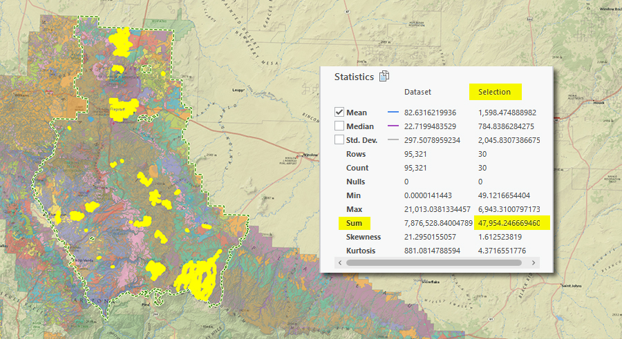
Neither sample is wrong. They answer different questions. Most of the polygons in this layer are small: the median polygon is 23 hectares, where the mean is 83. So a sample in which every polygon counts once is mostly small polygons, and the 30 selected that way average 60 hectares. But most of the land lies in the large polygons, so those polygons are a lot more likely to get sampled when every hectare counts. The 30 selected that way average 1,598 hectares, and even the smallest of them, at 49 hectares, is larger than the layer's median polygon. Select the first kind of sample when each polygon is equally important in your analysis, regardless of how large it is, and the second kind when you are trying to learn about the landscape in general.
The features are selected without replacement, by the method of Efraimidis and Spirakis (2006), which is equivalent to selecting one feature at a time, with each feature not yet chosen having a chance in proportion to its size. One consequence is worth knowing. Because no feature is selected twice, the largest features are chosen almost every time once the sample is a large share of the population, and their overall chance of selection is then no longer strictly in proportion to their size. The proportionality is closest when the sample is a small part of the whole (Efraimidis 2015).
Systematic selection
A systematic sample takes records at a regular interval, and it spreads the sample evenly through whatever order the records are put in. Sorted by date, it is even through time. Sorted by a station or a mile-marker number, it is even along the route.
The records of the population are first put in ascending order of the Sort field, which is the ObjectID field unless you choose another. Whole numbers, decimal numbers, text and dates can all be sorted on. Records with no value in the sort field come last when the field holds numbers, and first when it holds text or dates.
- Every Xth record takes one record in every X. With Random starting record checked, which is the default, the first one taken is chosen at random from among the first X, and every record then has the same one-in-X chance of being in the sample. Unchecked, the walk starts at the first record. Either way the sample comes to about the population divided by X.
- Odd-numbered and even-numbered records are every other record of that order, half the population each. The numbering is the record's place in the sorted order and has nothing to do with whether its ObjectID is an odd or an even number. There is nothing random in these two: the same records come out every time.
The population and the selection method
Every sample is selected from a population, and which records make up the population depends on the Selection method:
| Selection method | The population | What becomes of the sample |
|---|---|---|
| New selection | Every record. | It becomes the selection, replacing whatever was selected before. |
| Add to the current selection | The records that are not currently selected. | It joins the current selection. |
| Remove from the current selection | The records that are currently selected. | It is deselected. The rest of the selection stays. |
| Select subset from the current selection | The records that are currently selected. | It stays selected. The rest of the selection is dropped. |
The population is settled before anything is calculated, and that holds for every sampling method. A percentage is a percentage of the population. The calculated sample size takes the population's size as N. The areas and lengths are those of the population's features, and the systematic methods walk the population and nothing else. So removing 10% removes 10% of what is selected, and choosing even-numbered records under Add to the current selection selects every other one of the records that were not selected.
Some of what this makes easy:
- Thinning a selection. Select the features of interest by attribute or by location in the usual way, then run the tool with Select subset from the current selection to cut them down to a random sample of themselves.
- A second sample that cannot overlap the first. Run the tool, then run it again with Add to the current selection. The second sample is selected only from the records the first one left unselected.
- Two complementary sets. Select a percentage, copy the selection out (perhaps by exporting a subset of these selected features, or by making a new layer from the selected features), switch the selection, and copy again. The two copies share no records and together hold them all, which is the usual division into data for building a model and data for testing it.
Remove from the current selection and Select subset from the current selection need something to be selected, and stop with a message when nothing is.
Restricting the sample to an area
For a feature layer, the population can be limited to part of the map in two ways, which can be used together:
- An analysis extent, the rectangle set in the usual way: the current display, the extent of a layer, or a box drawn on the map.
- A polygon analysis boundary: a polygon layer from the map or a polygon feature class on disk. If the boundary layer has a selection, only its selected polygons form the boundary. With nothing selected, all of them do.
Features qualify when then says how a feature has to lie in order to count: Intersecting the extent or boundary, which is the default, takes every feature that touches the area, and Entirely within the extent or boundary takes only those that lie wholly inside it. For the second test the boundary polygons are merged first, so a feature that straddles two adjoining boundary polygons still counts as inside. When both an extent and a boundary are given, a feature has to pass both.
These limits combine with the selection method. Under Select subset from the current selection, for example, the population is the selected features that also lie in the area. A table has no geography, so for a table these three settings are not shown.
The examples earlier on this page use a polygon analysis boundary. The comparison of Fixed number of records with Fixed number, probability proportional to area / length selected its polygons inside the Coconino National Forest. There we chose Entirely within the extent or boundary, because we did not want to select TEU polygons outside the Coconino that merely touched its edge. The ranger district example selected points, which cannot reach across a boundary the way a polygon can, so Intersecting the extent or boundary served there.
Repeating a selection
Leave Random seed empty and every run selects a fresh sample. Give it a whole number and the same seed, with the same data and the same settings, gives the same sample every time. Report the seed with the methods and anyone can select the same sample again. Each run is also recorded, with all its settings, in the project's geoprocessing history.
Keeping the sample
A selection lasts only until something changes it. To keep the sample, copy the selected records to a dataset of their own with Copy Features, Copy Rows or Export Features, all of which act on the selected records of a layer.
You can also make a new layer that shows only the selected features. Right-click the layer in the Contents pane, go down to Selection, and choose Make Layer From Selected Features:
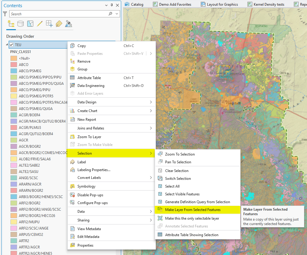
The new layer reads from the same dataset as the original and keeps a list of the features that were selected, so nothing is copied. Esri describes such a selection layer as a temporary working dataset: the list is of ObjectIDs, and it stops being right if the source data are changed. For a sample that has to last, copy it out.
To mark the sample without copying it, calculate a field while the sample is selected.
How it compares with the Esri tools
This tool complements other standard ArcGIS Pro random selection tools. The software currently has three that will randomly select from features or records in an existing dataset. Select Random Sample, in the Data Reviewer toolbox, is the one most similar to this tool: it applies a selection, as this tool does, but it needs the Data Reviewer extension. Subset Features, in the Geostatistical Analyst toolbox, splits a feature class or table at random into a training set and a test set, written as new datasets. Create Random Points, in the Data Management toolbox, makes new random points, but when it is given a point feature class to constrain it, it writes a random subset of those points to a new feature class instead.
| Select Random Records | Select Random Sample | Subset Features | Create Random Points | |
|---|---|---|---|---|
| What you get | A selection on the layer or table. | A selection on the layer or table, and an optional file listing the ObjectIDs chosen. | A new dataset holding the subset, and optionally one holding the rest. | A new point feature class holding the subset. |
| Input | A feature layer of any geometry, or a table view. | A feature layer or a table view. | A feature class or a table. | Point features only. |
| License | Every level, with no extension. | Requires the Data Reviewer extension. | Every level. | Every level. |
| Sample size | A fixed number, a percentage, a size calculated from a confidence level and margin of error, a number selected in proportion to area or length, or every Xth record. | A fixed number, a percentage, or the same calculated size. | A fixed number or a percentage. | A fixed number. |
| Larger features more likely | Yes, by geodesic area or length. | No. | No. | No. |
| Systematic selection | Every Xth, odd or even record in a sort order. | No. | No. | No. |
| Combining with a selection | The four standard methods, each with its own population. | Not a parameter of the tool. | Not a parameter of the tool. | Not a parameter of the tool. |
| Limiting the area | An analysis extent, a polygon boundary, or both. | Not a parameter of the tool. | Not a parameter of the tool. | Not a parameter of the tool. |
| Spacing between the chosen points | No. | No. | No. | A minimum distance can be set. |
| Repeating a selection | A random seed. | No seed. | Not a parameter of the tool. | The Random number generator environment. |
When the result should be a selection, this tool or Esri's Select Random Sample is the one to use. When it should be a new dataset, Subset Features does that in one step, and so does this tool followed by Copy Features or Copy Rows.
ModelBuilder
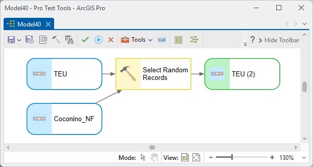
The tool has one derived output, Updated input (with the selection applied): the input layer or table view carrying its new selection. Connect it to Copy Features or Copy Rows and the model writes the sample out as a dataset. At the other end, the Recommended sample size that Estimate Sample Size produces can be connected to Number of records, so a sample size is never retyped between working it out and using it.
Parameters
| Label | Explanation | Data type |
|---|---|---|
| Input layer or table view (a selection is applied to it)Required · in_layer | The feature layer or table view to select from. It has to be a layer or a table in a map. A definition query on it is honored. | Feature Layer; Table View |
| Sampling methodRequired · sample_method | How the sample is chosen: Fixed number of records (the default), Percentage of records, Sample size calculated from a confidence level and margin of error, Fixed number, probability proportional to area / length, Systematic: every Xth record, Systematic: odd-numbered records or Systematic: even-numbered records. Only the settings the chosen method uses are shown. | String |
| Number of recordsOptional · n_records | The number of records to select, for the two fixed-number methods. It must be greater than zero. | Long |
| Percentage of records (0-100)Optional · percent | The percentage of the population to select: greater than 0 and no more than 100. | Double |
| Confidence level, percentOptional · confidence | How sure the estimate should be (default 95). It must be between 0 and 100. A higher level calls for a somewhat larger sample. | Double |
| Margin of error, percentOptional · margin | How far off the estimate may be, in percentage points (default 5). It must be between 0 and 100. Halving it takes four times the sample. | Double |
| Interval X (every Xth record)Optional · interval | X, for Systematic: every Xth record. It must be greater than zero. | Long |
| Sort field (systematic methods walk this order; defaults to the ObjectID field)Optional · sort_field | The field whose ascending order the three systematic methods walk. It is filled in with the ObjectID field when a systematic method is chosen. A whole-number, decimal, text or date field can be used. | Field |
| Random starting record (the first sample falls within the first X records)Optional · random_start | For Systematic: every Xth record. Checked (the default), the first record taken is chosen at random from the first X. Unchecked, the walk starts at the first record. | Boolean |
| Selection methodRequired · selection_method | New selection (the default), Add to the current selection, Remove from the current selection or Select subset from the current selection. The choice also decides the population the sample is selected from. See The population and the selection method. | String |
| Analysis extent (optional -- only features in this area are considered)Optional · extent | Limits the population to the features in this rectangle. Feature layers only. | Extent |
| Polygon analysis boundary (optional -- only features in these polygons are considered; a selection on the layer is honored)Optional · boundary | Limits the population to the features in these polygons. A selection on a boundary layer is honored. Feature layers only. | Feature Layer; Feature Class |
| Features qualify whenOptional · extent_relation | Intersecting the extent or boundary (the default) or Entirely within the extent or boundary. Enabled once an extent or a boundary is given. | String |
| Random seed (optional -- same seed, same selection)Optional · random_seed | A whole number that makes the selection repeatable. Left empty, every run selects a new sample. | Long |
| Updated input (with the selection applied)Derived · out_layer | The input layer or table view with its new selection, for connecting to the next tool in a model. | Feature Layer; Table View |
Python
A sample whose size is calculated from a confidence level and margin of error, made repeatable with a seed, and then copied out. The input is made into a layer first, because the tool selects on a layer and not on a dataset:
import arcpy
arcpy.ImportToolbox(r"C:\path\to\JennessEnterprisesTools.pyt")  # your install path
arcpy.management.MakeFeatureLayer(
    r"D:\data\study.gdb\veg_polygons", "veg_lyr")
arcpy.jenness.SelectRandomRecords(
    in_layer="veg_lyr",
    sample_method="Sample size calculated from a confidence level and margin of error",
    confidence=95.0, margin=5.0,
    selection_method="New selection",
    random_seed=42)
arcpy.management.CopyFeatures("veg_lyr", r"D:\data\study.gdb\veg_sample")
Recommended citation
Credits and references
By Jeff Jenness, Jenness Enterprises (www.jennessent.com). This tool belongs to the same family as Esri's Data Reviewer Select Random Sample tool, and shares its calculation of a sample size from a confidence level and margin of error. What it adds are selection in proportion to area or length, systematic selection, the four selection methods with their populations, limits by an extent or a polygon boundary, and a random seed for repeating a selection. It needs no extension.
- Efraimidis, P. S. 2015. Weighted random sampling over data streams. arXiv:1012.0256. arxiv.org/abs/1012.0256
- Efraimidis, P. S., and P. G. Spirakis. 2006. Weighted random sampling with a reservoir. Information Processing Letters 97:181–185. doi.org/10.1016/j.ipl.2005.11.003
- Efraimidis, P. S., and P. G. Spirakis. 2008. Weighted random sampling. In: Encyclopedia of Algorithms. Springer, Boston. doi.org/10.1007/978-0-387-30162-4_478
- Pennsylvania State University. STAT 506: Sampling Theory and Methods. Lesson 2, Confidence Intervals and Sample Size. Department of Statistics online course notes. online.stat.psu.edu/stat506/Lesson02
Licensing information
Works at every ArcGIS Pro license level (Basic, Standard, Advanced). No extension licenses are required.
Related tools and pages
- Estimate Sample Size — how many samples an accuracy assessment needs.
- Random Point Generator — makes new random points, where this tool samples features that already exist.
- Spatially Balanced Sample (GRTS) — a random sample that is also spread evenly over the study area.
- Repeating Shapes — tiles a study area with cells, from which this tool can keep a random subset.
- Voronoi (Thiessen) Polygons — another source of cells to sample from.
- Classification Accuracy (Kappa) — the assessment a verification sample feeds.
- About Kappa and classification accuracy analysis — designing an accuracy assessment.
- Attribute Summary Reports — counts, percentages and statistics of a layer's selected records.
- Load Favorite Datasets — add your most-used datasets to a map with one click.