Random Sample Array Generator

Geometric Tools · geoprocessing tool · by Jeff Jenness

Works at every ArcGIS Pro license level

Summary

Generates randomly placed arrays of sampling points — the standard field design of multiple sampling stations per plot — inside polygon features, along polyline features, within the data cells of an integer raster with an attribute table, or in a plain extent. Each array (a grid of rows and columns, a triangular lattice filling a circle, a circle of evenly spaced points, or a one-dimensional array along a polyline) is built around a randomly placed focal location using the Random Point Generator's stratified sampling design. Counts, the minimum distance between arrays, and the minimum distance from the boundary all refer to the arrays — footprints, nearest points, never centers. Arrays can be required to fit entirely inside the area or allowed to extend beyond it; the full array is generated either way. An optional seed makes runs exactly reproducible.

Why arrays instead of random points?

Mostly because of what a field day actually costs. Reaching a remote sample site is usually the expensive part — the drive, the hike, the navigation — while moving to the next station within an array is comparatively cheap. The sampling itself may be no small matter: a team of specialists — botanists, mammalogists, entomologists, hydrologists — can spend hours working a single station. But that effort is the same under either design; what changes is the travel wrapped around it. A design of scattered single points pays the full approach cost for every station, while an array pays it once and then reaches its neighboring stations in a short walk. If getting to a site takes two hours and the next station in the array is fifty meters away, a 25-station array buys twenty-five stations for roughly one approach — the scattered design pays twenty-five.

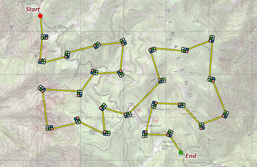
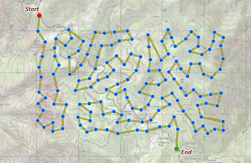
The two routes below make the point on real ground: the same 150 stations, the same start and end, both visit orders estimated with the same shortest-path heuristic that powers our Estimated Shortest Path through Points tool — 22.4 km of travel when the stations are grouped into 25 arrays, against 40.4 km when they are scattered singly. The scattered design walks 1.8 times as far to collect the very same number of measurements. And whichever design you choose, if you plan to hike to each station, that tool will hand you an efficient field survey route of your own — often a substantial saving in overall effort and time.

A topographic map with a survey route from a Start point through 25 clustered arrays of 6 points each to an End point; the route strides efficiently between the arrays — 150 stations in 25 arrays: **22.4 km** from Start to End.

The same map with a survey route through 150 scattered single points; the route wanders back and forth across the entire area — The same 150 stations scattered singly: **40.4 km** — 1.8 times the walk.

The catch is spatial autocorrelation: stations a few dozen meters apart tend to echo one another, so 100 points packed into 4 arrays carry fewer independent facts than 100 points scattered singly. The classic accounting uses the within-array correlation ρ: with g arrays of m points each, the effective number of independent samples is approximately

n_{eff} = \frac{g m}{1 + (m - 1) ρ}

At ρ = 0 every station counts in full; at ρ = 1 each array collapses to a single independent fact. In between, the tax is real: 4 arrays of 25 points with ρ = 0.3 are worth about 12 independent points, not 100. If the goal is simply a landscape mean, that is the trade — and arrays still often win it, because travel usually costs far more than the correlation takes.

But spatial autocorrelation can also be a good thing!

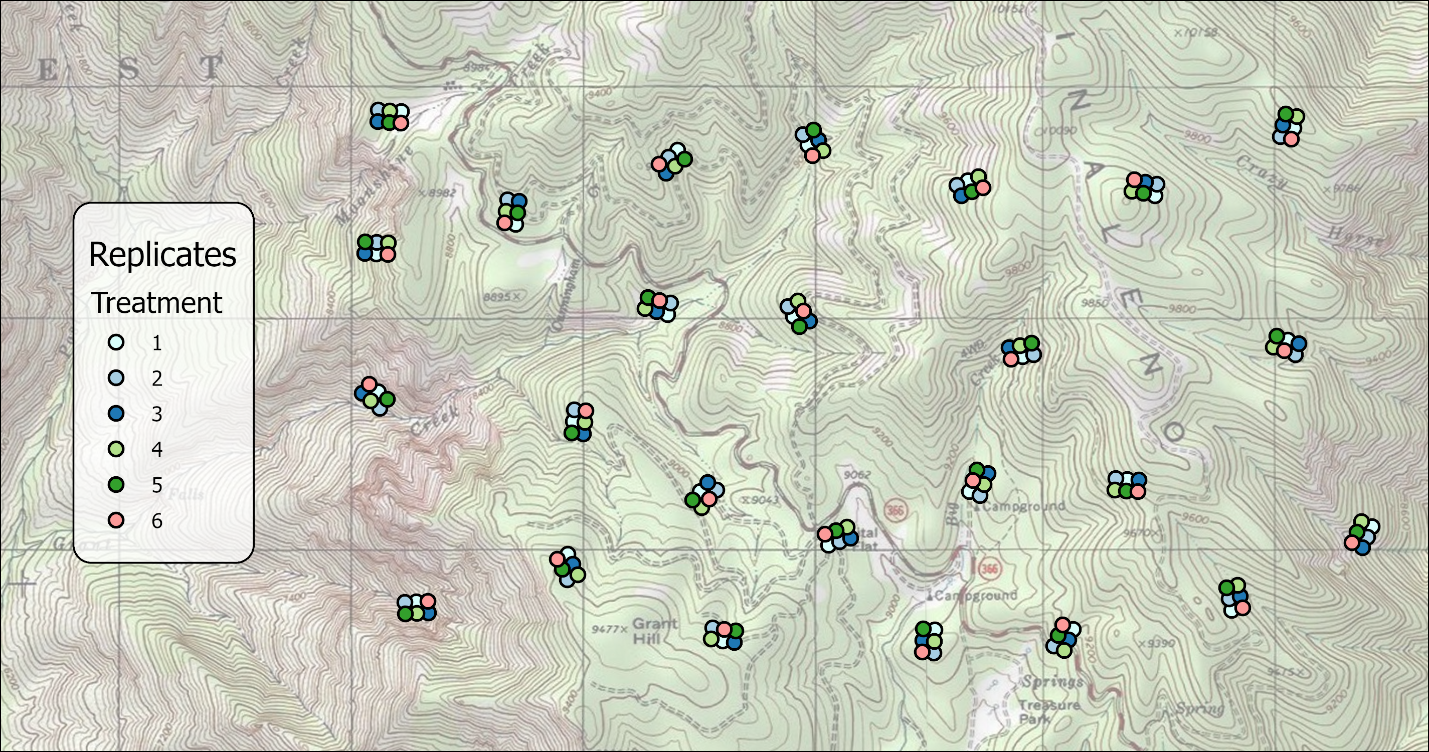
The correlation can be turned from a tax into the design's engine. Because the stations of one array share nearly constant environmental conditions, the array is a natural block: assign a different test condition to each station within the array — trap types, bait or lure treatments, survey methods, call-playback variants — and compare them where the environment is held still. Writing station j’s measurement in array i as the sum of an overall mean, its condition's effect τ_j, the array's shared environmental effect b_i, and noise,

y_{i j} = μ + τ_{j} + b_{i} + ε_{i j}

the comparison of two conditions within the same array is

y_{i A} - y_{i B} = τ_{A} - τ_{B} + (ε_{i A} - ε_{i B})

— and notice what is missing: b_i, the environmental condition of that array, has cancelled exactly. The very correlation that shrank n_eff is what guarantees the two conditions were tested under the same circumstances. The randomly placed arrays then do the other half of the work: each one drops the same set of conditions into a different, randomly drawn slice of the landscape, so the comparison is repeated across the full range of environments rather than the one place you happened to stand. This is Fisher's classic randomized block design wearing field boots — the array is the block, the stations are the plots — and it is why the honest sample count for this tool is the number of arrays.

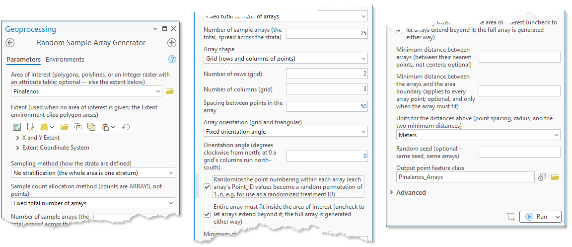
One option exists precisely for this design: Point_ID normally follows the array's geometry, so a treatment keyed to Point_ID would sit at the same position in every array — confounding treatments with position effects (edge stations, the center, the north corner). Check Randomize the point numbering within each array and each array's Point_ID values become a fresh random permutation of 1..n instead, reproducible with the seed — the same treatments in every block, at freshly randomized stations, exactly as Fisher would insist.

A topographic map with 25 replicate arrays of six points, each point colored by Treatment 1 through 6; the six colors appear once in every array but in a different arrangement each time — The blocking design on the ground: six treatments in every replicate array, their positions freshly randomized within each array — identical experiments dropped into 25 randomly drawn environments.

Usage

This tool is the Random Point Generator's companion: the same areas of interest, the same stratified sampling design, the same reproducibility seed — but each sample is an array of points built around a randomly placed focal location, the standard design when every plot carries multiple sampling stations: vegetation subplots around a plot center, point counts along a transect, pitfall traps on a grid. One number to hold onto throughout: if you ask for 4 arrays of 25 points each, the sample count is 4.

The Geometric Tools gallery open on the ribbon, with the Random Sample Array Generator button, in the Random Samples row, outlined in blue — Where to find it: **Random Sample Array Generator** is in the *Random Samples* row of the *Geometric Tools* gallery, in the Geometric Tools group of the *Wildlife and Forestry* tab.

The area of interest

Polygons (selections honored, holes respected), polylines, an integer raster with an attribute table (NoData excluded), or a plain extent. For polygons, rasters and extents the focal location is drawn uniformly by area and the array is built around it. For polylines the focal location is drawn uniformly along the lines, and the array either surrounds it in two dimensions (grid, triangular, circular) or runs along the line itself — the one-dimensional shape below.

The four array shapes

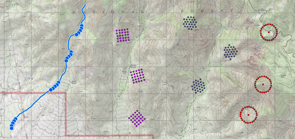
Grid — rows × columns at a point spacing, in a square pattern. Every point carries its Row and Col (1-based; row 1 is north and column 1 west at zero orientation).
Triangular — the requested number of points on a triangular lattice, taken in order of increasing distance from the focal point (ties resolved by azimuth, so seeds reproduce exactly); with many points the array fills a circle. Point 1 is the focal point itself.
Circular — points evenly spaced on a circle of the given radius: 12 points at 100 m sit 30° apart, each 100 m from the focal point, and each carries its Bearing. The first point lies due north unless the random starting angle option spins the whole ring by a random fraction of one step. The center point can be included as a sample point (the classic center-plus-satellites cluster plot), in which case it counts toward the point total — 12 points = the center plus 11 on the circle.
Along the polyline (polylines only) — a one-dimensional array of points at a fixed interval along the line, centered on the focal location: an odd count puts a point exactly there, an even count straddles it. The walk continues straight through junctions it passes; when it reaches the end of a line where more than one continuation exists (a Y confluence), one branch is picked and a warning reports how many arrays did so; a dead end that would cut the array short rejects the placement, and the tool draws a new focal location instead.

The Random Sample Array Generator dialog set to place 25 grid arrays of 2 by 3 points at 50-meter spacing, with the randomize-point-numbering and entire-array-must-fit options checked — A grid design: 25 arrays of 2×3 points at 50 m spacing, with the point numbering randomized within each array so Point_ID can serve as a treatment ID, and every array required to fit inside the area of interest.

A topographic map with all four array shapes placed on it: a one-dimensional array of points along a stream in blue, square grid arrays in magenta, triangular arrays in dark blue, and circular arrays with their center points in red — All four shapes over the same country: one-dimensional arrays walking a stream (blue), randomly oriented grids (magenta), triangular arrays (dark blue), and circular plots with their center points included (red).

Orientation

Grid and triangular arrays take a fixed angle (degrees clockwise from north; at zero a grid's columns run north-south), a fresh random angle for every array, or — on polylines — alignment to the local line direction, so the rows run along the stream or transect the array sits on. Circular arrays are direction-free; their randomization is the starting angle above.

Everything refers to the arrays, not the points inside them

The sampling method and allocation counts count arrays. The minimum distance between arrays is measured between their nearest points — footprints — so two arrays can never approach closer than the minimum anywhere, not merely center-to-center. On polylines that distance can be measured spatially, along the line, or through the connected network, exactly as in the Random Point Generator (whose page tells the drainage-bottoms story behind the three choices). And the minimum distance from the area boundary applies to every point of the array, not just its center.

When an array does not fit

With Entire array must fit checked — the default — a placement whose array would leave the polygon, land on NoData cells, or run off the end of a line is rejected and a new focal location is drawn, so every delivered array is complete; most ecological designs require exactly that for consistent sampling. Unchecked, arrays may extend beyond the area of interest: the full array is still generated, raster points beyond the data carry a null Category, and the boundary-distance constraint no longer applies. The Advanced placement-attempts budget bounds how hard the tool tries per array before accepting a shortfall — containment rejections and spacing conflicts both consume attempts. And a design that cannot possibly fit (an array wider than the polygon, raster or line network can hold) is detected up front and reported immediately, without consuming the budget at all.

Stratified sampling

Stratification follows the Random Point Generator exactly: strata are individual polygons or polylines, raster categories, contiguous raster regions, or groups sharing a strata ID value; array counts are allocated equally, proportionally to stratum area or length, from a population field, or by density (arrays per acre, hectare, square kilometer — or per length of line). Geodesic areas and lengths keep the allocation honest in any coordinate system, and geographic data is handled in an automatic equal-area working projection — arrays are built in true meters and written back in the input coordinate system.

Output and reproducibility

The output is a point feature class with Array_ID and Point_ID (the sequence within its array), plus Row/Col for grids, Bearing for circles, and the usual Stratum, Src_FID and Category fields where they apply — everything needed to navigate to station 7 of plot 3. The random seed makes runs exactly reproducible: the same inputs with the same seed give the same arrays. Cite it in a methods section.

ModelBuilder

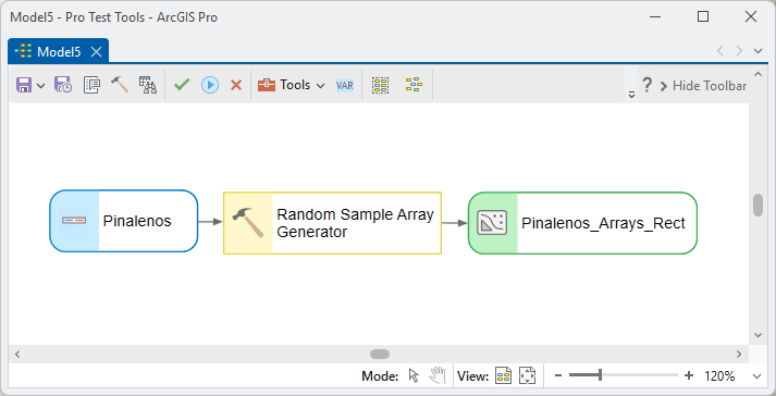
The output point feature class chains directly into whatever comes next, and the array count can chain in from upstream — Estimate Sample Size's derived recommendation feeding the number-of-arrays parameter:

Parameters

Label	Explanation	Data type
Area of interestOptional · boundary	Polygons, polylines to place arrays along, or an integer raster with an attribute table (NoData excluded). Selections are honored. Leave blank to use the extent parameter instead.	Feature Layer; Raster Layer
ExtentOptional · extent	A plain rectangular area, used when no area of interest is given.	Extent
Sampling method (how the strata are defined)Required · strata_method	No stratification; each individual polygon or polyline; each raster category; each contiguous raster region; or groups sharing a strata ID value. Identical to the Random Point Generator, phrased to match the input.	String
Strata ID fieldOptional · strata_field	The integer or text field whose values group features or raster categories into strata. The ObjectID field also qualifies.	Field
Sample count allocation methodRequired · alloc_method	How many arrays each stratum receives: an equal count, a count proportional to stratum area (or length), a count equal to or proportional to a population field, or a density of arrays. The counts are arrays — 4 arrays of 25 points each is a count of 4.	String
Number of sample arraysOptional · n_arrays	The overall number of arrays, distributed across the strata (proportional methods) or the whole area.	Long
Number of sample arrays per stratumOptional · n_per_stratum	The number of arrays each stratum receives (equal-count allocation).	Long
Population fieldOptional · population_field	A non-negative numeric field driving the equal-to or proportional-to population allocations.	Field
Density: arrays per unitOptional · density	How many arrays per unit — e.g. 0.1 arrays per square kilometer. Counts come from geodesic areas and lengths.	Double
Density unitOptional · density_units	Acre, Square Mile, Hectare or Square Kilometer for areas; Foot, Mile, Meter or Kilometer of line length for polylines.	String
Array shapeRequired · array_shape	Grid (rows and columns at a point spacing); Triangular (a lattice filling a circle); Circular (points evenly spaced on a circle, optionally including the center); or Along the polyline (one-dimensional; polylines only).	String
Number of rows (grid)Optional · n_rows	Grid arrays: the number of rows. Row 1 is the northernmost at zero orientation.	Long
Number of columns (grid)Optional · n_cols	Grid arrays: the number of columns. Column 1 is the westernmost at zero orientation.	Long
Number of points in each arrayOptional · array_points	Triangular, circular and along-the-line arrays: how many points each array contains. For circular arrays with the center included, the center counts — 12 points = the center plus 11 on the circle.	Long
Spacing between points in the arrayOptional · point_spacing	The distance between neighboring points within each array (grid, triangular and along-the-line shapes), in the units below.	Double
Circle radiusOptional · radius	Circular arrays: every point sits exactly this far from the focal point, in the units below.	Double
Array orientation (grid and triangular)Optional · orientation_mode	A fixed orientation angle; a fresh random angle for each array; or alignment to the polyline direction at the focal location (polylines only).	String
Orientation angleOptional · orientation_angle	The fixed rotation of every array, degrees clockwise from north. At zero a grid's columns run north-south and its rows east-west.	Double
Random starting angle for the first point on the circleOptional · randomize_start	Circular arrays: spin the whole ring by a random fraction of one step, so the first point falls anywhere within the first step instead of due north. The seed controls the spin.	Boolean
Include the center point as a sample pointOptional · include_center	Circular arrays: also place a sample point at the focal location itself. The center counts toward the number of points.	Boolean
Randomize the point numbering within each arrayOptional · randomize_ids	Checked: each array's Point_ID values become a fresh random permutation of 1..n (reproducible with the seed), so Point_ID can serve as a randomized treatment ID. Row/Col and Bearing still describe the geometric position; Point_ID 1 is then no longer the focal or center point.	Boolean
Entire array must fit inside the area of interestOptional · must_fit	Checked (default): placements whose arrays would leave the polygon, land on NoData, or run off a line are rejected and redrawn — every delivered array is complete. Unchecked: arrays may extend beyond the area; the full array is still generated, and the boundary distance no longer applies.	Boolean
Minimum distance between arraysOptional · min_spacing	No two arrays will approach closer than this anywhere — measured between their nearest points (footprints), never between centers.	Double
How the minimum distance is measuredOptional · spacing_type	Polylines only: absolute spatial distance, distance along the polyline, or network distance through connected lines — the same three choices as the Random Point Generator.	String
Minimum distance between the arrays and the area boundaryOptional · boundary_gap	Every point of every array stays at least this far inside the boundary (from polygon edges and holes; from NoData/edge cells on rasters; measured along the line beyond the array's end points on polylines). Available only when the entire array must fit.	Double
Units for the distances aboveOptional · linear_units	Units for the point spacing, the circle radius, and the two minimum distances: Meters, Kilometers, Feet or Miles.	String
Random seedOptional · random_seed	The same seed with the same inputs reproduces the same arrays exactly. Leave blank for a fresh draw each run.	Long
Placement attempts per arrayOptional · max_attempts	Advanced: how many candidate focal locations each array may consume before the tool gives up on reaching the full count (default 1000). Containment rejections and spacing conflicts both consume attempts.	Long
Output point feature classRequired · out_fc	The output points: Array_ID, Point_ID (the sequence within its array), Row/Col for grids, Bearing for circles, and the usual Stratum, Src_FID and Category fields where they apply.	Feature Class

Python

Five 5×5 grid plots at 50 m spacing, at least 500 m apart, each fitting entirely inside the study area, reproducible with a seed (the comment block lists every option string — matching is by prefix):

import arcpy
arcpy.ImportToolbox(r"C:\path\to\JennessEnterprisesTools.pyt")  # your install path
# strata_method options (matching is by prefix; same as Random Point Generator):
#   "No stratification (the whole area is one stratum)"
#   "Stratify by individual polygon" / "... polyline"
#   "Stratify by raster category (Value field)"
#   "Stratify by contiguous raster region"
#   "Stratify by strata ID field"  (+ strata_field)
# alloc_method options (counts are ARRAYS):
#   "Fixed total number of arrays"  (unstratified)
#   "Equal count in each stratum"  (+ n_per_stratum)
#   "Count proportional to stratum area" / "... length"
#   "Count equal to a population field" / "Count proportional to a population field"
#   "By density (arrays per area unit)" / "... per length unit"
# array_shape options:
#   "Grid (rows and columns of points)"  (+ n_rows, n_cols, point_spacing)
#   "Triangular (a triangular lattice filling a circle)"  (+ array_points, point_spacing)
#   "Circular (points evenly spaced on a circle)"  (+ array_points, radius,
#       randomize_start, include_center)
#   "Along the polyline (a one-dimensional array of points)"  (+ array_points,
#       point_spacing; polylines only)
# orientation_mode: "Fixed orientation angle" / "Random orientation for each array" /
#   "Align each array to the polyline direction"  (polylines only)
# spacing_type: "Absolute spatial distance" / "Distance measured along the polyline" /
#   "Network distance through connected polylines"
# linear_units: "Meters" / "Kilometers" / "Feet" / "Miles"
arcpy.jenness.RandomSampleArrayGenerator(
    boundary=r"D:\data\study.gdb\study_area",
    strata_method="No stratification (the whole area is one stratum)",
    alloc_method="Fixed total number of arrays",
    n_arrays=5,
    array_shape="Grid (rows and columns of points)",
    n_rows=5, n_cols=5, point_spacing=50.0,
    orientation_mode="Random orientation for each array",
    must_fit=True, min_spacing=500.0,
    linear_units="Meters", random_seed=42,
    out_fc=r"D:\data\study.gdb\sample_arrays")

Recommended citation

Jenness, J. 2026. Random Sample Array Generator. Wildlife and Forestry Tools add-in for ArcGIS Pro, v. 1.81 (August 2026). Jenness Enterprises. Available at: https://github.com/JeffJenness/Wildlife_Tools.

Credits

By Jeff Jenness, Jenness Enterprises (www.jennessent.com). A companion to the author's classic Random Point Generator (randpts.avx) extension, generating arrays of sampling stations with its stratified sampling design.

Licensing information

Works at every ArcGIS Pro license level (Basic, Standard, Advanced). No extension licenses are required.

Random Point Generator — single random points on the same chassis: same areas of interest, strata, allocation, spacing types and seed.
Repeating Shapes — systematic point patterns over the whole area, when the stations should not be random.
Estimate Sample Size — how many samples the design needs; its derived count feeds the number of arrays in ModelBuilder.
Select Random Records — random selection from features that already exist.
Estimated Shortest Path through Points — the tool behind the route figures above; order your stations into an efficient field survey route for hiking to every one.
Radiating Lines and Points — a ring of sampling locations at a fixed distance and regular bearings around every station, with optional barriers.