

About Kappa and Classification Accuracy Analysis
Introduction
Spatially explicit models have various applications in resource management, including the development of vegetation and wildlife habitat relationship predictive surfaces. Appropriate applications of these models are impossible without informed approaches to model development and accuracy assessment of the resulting data products. In the absence of incisive model development and error analysis, spatially explicit models may be applied in ways that confound, rather than illuminate, our understanding of vegetation land cover and wildlife habitat.
Accuracy assessment provides a means of gauging model performance, and end users who conduct accuracy assessments gain important information regarding model reliability and the suitability of the modeling process. Following Congalton and Green (1999), accuracy assessments are useful for: (1) ascertaining the quality of a predictive surface; (2) improving classification quality by identifying and correcting sources of error; (3) facilitating comparisons of algorithms, techniques, model developers and interpreters; and (4) determining the relevance of the data product in the decision-making process.
When accuracy assessments are conducted at all, generally only the overall accuracy metric is provided — yet the error matrix behind that single number supports a rich family of statistics that describe model performance far more completely. This page walks through that family: the error matrix itself, overall, user's and producer's accuracies, the Kappa statistic with its variance and tests, the per-class diagnostic metrics, the class-proportion weighting that turns an accuracy assessment into an unbiased area estimator, and the modern statistics that today's journals expect. The Classification Accuracy (Kappa) tool computes everything described here; this page explains what the numbers mean and where they come from.
The error matrix
The foundation of nearly everything on this page is the error matrix (also called a confusion matrix or contingency table). Each reference sample contributes to exactly one cell: the cell at row i, column j counts the sample points that were predicted to be class i and observed in the field to be class j. The diagonal (where i = j) represents cases where the predicted value agreed with the observed value; the off-diagonal cells contain the misclassifications, and their row and column describe exactly how each value was misclassified.
| Observed (reference) class | |||||
|---|---|---|---|---|---|
| 1 | 2 | … | k | ||
| Predicted class |
1 | n11 | n12 | … | n1k |
| 2 | n21 | n22 | … | n2k | |
| … | … | … | … | … | |
| k | nk1 | nk2 | … | nkk | |
Overall, producer's and user's accuracy
The overall accuracy is simply the total number of correct classifications divided by the total number of sample points — the sum of the diagonal over the matrix total.
A useful companion to overall accuracy is the no-information
rate: the accuracy you could achieve by ignoring the samples
entirely and always guessing the commonest reference class. In the
tutorial dataset the commonest class is Oak/Juniper, at 133 of the
362 reference samples, so a “classifier” that mindlessly
labeled every sample Oak/Juniper would score
133 / 362 = 36.7% — no imagery, no
predictors, no effort. That number is the floor any real
classification must beat, and the report tests whether yours does
(a one-sided exact binomial test of overall accuracy against the
no-information rate, following the convention of R's
caret package). Read it as a sanity floor rather than a
high bar: failing it means the classification is extracting no usable
information from its predictors, while passing it says nothing about
whether the accuracy is good enough for your purposes. The rate
itself deserves a glance too — the more imbalanced the
landscape, the higher the floor sits, and the more flattering a raw
overall accuracy can look, a theme that returns with force in
the Kappa debate below.
Overall accuracy is often the only accuracy statistic reported with predictive landscape models, but the error matrix provides the means to calculate two further accuracies for each class — and these per-class accuracies are often more interesting to researchers than the overall figure, since a study species usually cares about particular classes rather than the classification as a whole. Indeed, the modern critics of summary statistics recommend the per-class accuracies as the centerpiece of the report (see the Kappa debate below). The distinction between the two matters:
- The producer's accuracy of class j is njj / n+j — of the samples observed to be class j, the proportion the classification got right. It answers: how well can this landscape be classified?
- The user's accuracy of class i is nii / ni+ — of the samples predicted to be class i, the proportion that really were. It answers: how reliable is the classification to the person using it? (Story and Congalton 1986)¶.
The difference is best understood with an example. Consider this error matrix of 136 sample points over three vegetation classes:
| Reference data | |||||
|---|---|---|---|---|---|
| Deciduous Forest | Coniferous Forest | Grassland | Total | ||
| Classification data |
Deciduous Forest | 60 | 22 | 4 | 86 |
| Coniferous Forest | 2 | 30 | 3 | 35 | |
| Grassland | 1 | 4 | 10 | 15 | |
| Total | 63 | 56 | 17 | 136 | |
The overall accuracy is (60 + 30 + 10) / 136 = 73.5%. But suppose we are interested specifically in deciduous forest. The reference data include 63 cases identified as deciduous forest, and 60 of them were correctly classified — a producer's accuracy of 95.2%, suggesting deciduous forest is captured very well. Notice, however, that 86 cases were classified as deciduous forest, so a “deciduous forest” label from the classification is correct only 60 / 86 = 69.8% of the time. Although the class can be classified with high accuracy from the producer's perspective, the actual reliability of the classification to the user may be much different — and both numbers deserve reporting.
The Kappa statistic
The Kappa statistic measures the agreement between two sets of categorizations of a dataset while correcting for chance agreement between the categories. Even a random classification would agree with the reference data some of the time, simply because both sides use the same classes in similar proportions; Kappa asks how much of the observed agreement exceeds that chance level. Following Congalton and Green (1999:50):
with its variance estimated by the delta method — the θ1 through θ4 formulation of Fleiss, Cohen and Everitt (1969), where each θ term is computed directly from the matrix counts and marginals:
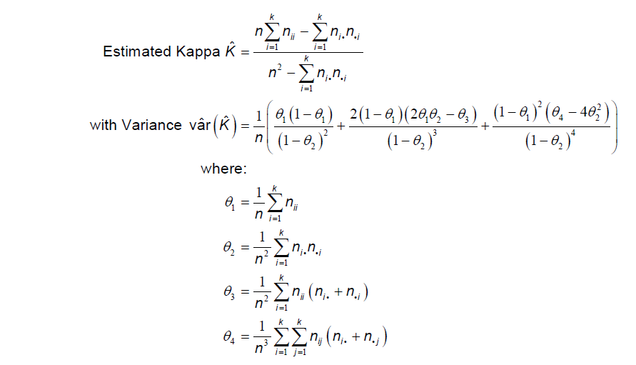
The logic of the chance correction can be summarized as follows (after Agresti 1990:366–367)¶. If Πo is the overall probability of correctly classifying a point (the overall accuracy), and Πe is the probability of agreement that would occur if the predicted and observed classifications were statistically independent — agreement purely by chance, computed from the products of the marginal proportions — then Πo − Πe is the excess accuracy beyond chance, and Kappa divides it by the excess that a perfect classification would have achieved:
typically ranges between 0 and 1, with values closest to 1 reflecting the highest agreement; negative values are possible but rare. For the example matrix above, = 0.53 — the classification performs 53% better than chance alone would.
Variance, significance tests and confidence intervals
Because is asymptotically normally distributed, and because its variance can be estimated from the matrix (the formulation shown above), three important inferences follow:
- A Z-test against chance: Under the null hypothesis K = 0, the classification is no better than random; a significant Z rejects that in favor of (hopefully) better-than-random accuracy.
- A confidence interval:
- Comparisons between analyses: because each analysis carries its own variance, two Kappas may be tested for equality with — useful for asking whether different models, methodologies or interpreters produce significantly different results, or whether a landscape has changed over time (Congalton and Mead 1983)¶. The comparison extends to any number of analyses through the variance-weighted common Kappa and its chi-square test of equality (Fleiss 1981:222)¶.
One further test in the report deserves its own introduction: the McNemar–Bowker marginal-symmetry test (McNemar 1947¶; Bowker 1948¶), which asks a question none of the statistics above ask — not how much the classification errs, but whether its errors are directionally biased. Under the null hypothesis the mistakes are an even trade — the misclassifications mirror each other: for every pair of classes, about as many samples get misclassified from class A into class B as from B into A, and consequently the classification's class totals agree with the reference totals apart from sampling noise. (Note this is symmetry of counts, not of per-stand error rates — when one class is far commoner than the other, an even trade of counts actually means the rarer class is erring at the higher rate.) The statistic is built from the off-diagonal cells alone — each pair of classes contributes (nij − nji)² / (nij + nji) — on k(k − 1)/2 degrees of freedom, and for two classes it reduces exactly to McNemar's original paired test. A significant chi-square says at least one pair of classes is trading samples predominantly one way. (Strictly, one-way flows around a cycle of three or more classes could cancel in the totals, but that is a curiosity; in practice the asymmetry shows up as classified totals that differ from the reference.) In the tutorial dataset, for example, the classification claims 174 samples' worth of Mixed Conifer where the observer found 130, while shorting Pine/Oak 35 to 52 — and the test (chi-square 31.85 on 6 df, P = 0.00002) confirms that imbalance is real bias, not luck. This is the inferential cousin of the quantity disagreement component described below, and it is an early warning that the classification's raw acreages are biased — precisely the problem the error-adjusted area estimates correct. When the test is not significant, the classification's class proportions are statistically defensible as drawn, and most of whatever error exists is allocation — right amounts, wrong places.
Why would you want to know this about your classification method? Because the two outcomes describe different diseases, calling for different remedies. Symmetric errors mean the method is fuzzy but fair: it confuses two classes, but guesses evenhandedly when it does, so no acreage flows systematically from one class into another. The only real cure for fuzziness is better discrimination — better training data for the confusable pair, an additional predictor variable, imagery from a season when the classes separate — and adjusting thresholds will not help, because the amounts are already right. Asymmetric errors mean the method is slanted: something systematic — an over-generous decision threshold, training data that let a dominant class swamp its neighbors, a one-way spectral resemblance — is pushing acreage in a preferred direction, and everything downstream that consumes areas inherits the bias. Here recalibration genuinely helps, and the direction of the asymmetry tells you which way to lean: in the tutorial dataset the classification converts Pine/Oak into Mixed Conifer at five times the reverse rate, which smells like sparse pine-oak canopy reading as conifer, and says plainly that Mixed Conifer's signature needs reining in. Even before anything is fixed, a slanted classification errs predictably, which is itself usable: a manager who knows Pine/Oak is systematically swallowed knows the classified extent is a floor, not an estimate. One caution, in the spirit of Tukey's objection below: the P value only says the lean is real, not that it is large — with enough samples even a trivial lean turns significant — so read the size of the margin gaps and the quantity-disagreement share first, and the P value second.
Cohen's three independence assumptions — and what breaking them costs
Cohen (1960)¶ laid down three independence assumptions for the statistic, and it is worth being precise about them, because the obvious worry — two observers rating the same points — is not a violation at all. Two judges categorizing the same sample of units is Cohen's design, not a breach of it. What he actually requires is independence of three other things, and each one, when violated, pushes the statistics in its own direction:
- The judges operate independently. This is about the judgment process: the field crew must record what they find without consulting the classification, and the classifier must not have been trained on the reference points. Violate it and agreement is partly copying, not concordance — kappa is biased upward. (This is why the tutorial's field protocol says to record the class independently of what the classification claims: using the classification to navigate to a point is fine; letting it whisper the answer is not.)
- The units are independent. The sample points should be independent draws from the landscape — the assumption real designs strain most, through spatial autocorrelation and systematic sampling: neighboring points share both vegetation and classification errors, so n points carry fewer than n independent facts (one of Congalton's 1991 core considerations). The point estimates remain essentially unbiased, but every variance is underestimated — confidence intervals too narrow, tests overconfident, P values too small. Spreading samples helps; beyond that, the honest posture is humility about borderline P values. (The bootstrap does not rescue you here, since it too resamples units as if they were independent.)
- Categories are mutually exclusive and exhaustive. Ecotones and mixed cells strain this: a cell that is half one class must be forced into one box, and the observer may lawfully force it into the other. Definitional disagreements then masquerade as classification error — kappa and the accuracies are biased downward. The circle-majority option treats the locational flavor of this; the definitional flavor is a classification-scheme problem no statistic fixes.
The same-points worry does surface in one legitimate place: not within either observer's analysis, but when their two kappas are compared. Kappas computed from overlapping samples are positively correlated, and the pairwise Z test ignores that covariance, overstating the variance of the difference — so the comparison runs conservative (see the Compare Accuracy Analyses page). Notice the tidy symmetry: violating unit independence within an analysis makes its tests overconfident, while sharing units between analyses makes their comparison underconfident — the same root cause, pushing in opposite directions depending on where the correlation lives. In both cases the point estimates survive; it is always the uncertainty statements that take the damage.
Per-class statistics: the confusion-matrix family
Several further metrics describe model performance for each class, derived by collapsing the error matrix to a 2×2 confusion matrix for that class — the four possible ways a sample may be classified and observed:
| Observed X | Observed not-X | |
|---|---|---|
| Classified X | a | b |
| Classified not-X | c | d |
- Sensitivity = a / (a+c) — equivalent to producer's accuracy: of the samples observed to be class X, the proportion the classification got right. It answers: how well can this landscape be classified? A sensitivity of 0.88 means the classification finds 88% of the real class X out there.
- Specificity = d / (b+d): of the samples observed not to be X, the proportion the classification correctly left unlabeled. A highly specific classification rarely claims X where X is absent.
- Commission error (false positive rate) = b / (b+d) = 1 − specificity: how often the classification commits the sin of claiming X on ground that is not X — the error its user walks into.
- Omission error (false negative rate) = c / (a+c) = 1 − sensitivity: the proportion of real X the classification omits. If X is critical habitat, this is the error that hides it from you.
- Positive predictive power = a / (a+b) — equivalent to user's accuracy: of the locations the classification labels X, the proportion that really are X. It answers: how reliable is the classification to the person using it? A value of 0.66 means one in three locations labeled X will disappoint the visitor.
- Negative predictive power = d / (c+d): of the locations the classification labels not-X, the proportion that truly are not — how far its absences can be trusted, which for survey planning is often the more expensive mistake.
The modern additions complete the family that R's
caret package reports, and each earns its keep:
- F1 = 2a / (2a+b+c): the harmonic mean of user's and producer's accuracy — one number per class that balances the two error directions, and punishes a classification that buys one accuracy at the expense of the other. It is the per-class score the species-distribution-modeling and machine-learning literatures report.
- Prevalence = (a+c) / n: the proportion of the reference samples that are class X — how common the class actually is, and the context every other number needs. An impressive specificity means little for a class with 1% prevalence, since almost everything is a true negative by default.
- Detection rate = a / n: the share of all samples that are correctly identified X — the class's contribution to the overall accuracy.
- Detection prevalence = (a+b) / n: the share of all samples the classification labels X. Compare it with prevalence to see at a glance whether the classification over-claims or under-claims the class: one that labels 48% of the ground as a class occupying 36% of the reference data is over-claiming it.
- Balanced accuracy = (sensitivity + specificity) / 2: the accuracy you would see if X and not-X were equally common — a guard against the flattery of dominant classes, and a fairer single number when prevalence is far from 50%.
For detailed treatments of these concepts, the classic guide to the
sensitivity/specificity family in ecological modeling remains Fielding
and Bell (1997)¶. The modern additions carry their own literature: the
F-measure descends from information retrieval (Van Rijsbergen 1979)¶;
Sokolova and Lapalme (2009)¶ give formal definitions for the family
and — more usefully — work out which changes in the error
matrix each measure is blind to; their observation that precision,
recall and F1 never see the correct absences is exactly why the
report pairs F1 with specificity, negative predictive power and
balanced accuracy rather than letting it stand alone.
Allouche, Tsoar and Kadmon (2006)
examine how prevalence distorts kappa in species-distribution models
and champion the prevalence-independent true skill statistic as the
alternative (their TSS = sensitivity + specificity − 1
is a simple rescaling of the balanced accuracy reported here:
TSS = 2 × balanced accuracy − 1);
Brodersen et al.
(2010)¶ formalize balanced accuracy; and Kuhn (2008)¶ documents the
caret package whose report these statistics mirror.
Weighted-average versions over all classes are computed by summing the
per-class confusion matrices into one overall matrix; the per-class
conditional Kappa (Congalton and Green 1999) applies the same
chance correction classwise, with its own standard error.
Designing the assessment
Classification considerations
The choice of classification system can greatly influence the measured accuracy. Congalton (1991)¶ offers guidelines worth restating: (1) all areas to be classified should fall into one and only one category; (2) all areas should be classified — none left unclassified; (3) where possible use a hierarchical system, so categories can be collapsed into more general ones if the original set cannot meet your accuracy requirement; and (4) recognize that standard class breakpoints may be arbitrary — if your data cluster around a breakpoint (say, a canopy-closure class boundary), natural breaks may serve you better. (The Fisher-Jenks natural-breaks algorithm is built into ArcGIS Pro's own symbology tools — the “Natural Breaks (Jenks)” classification in any layer's symbology pane — so identifying sensible breakpoints takes nothing beyond the standard software.)
Sample point considerations
As a general rule of thumb, Congalton and Green recommend a minimum of 50 sample points per category, increasing to 75–100 per category with large numbers of categories (more than about 12). This may be an obvious point, but under no circumstances should you completely fail to sample any category — it is difficult to estimate the classification accuracy of a category you never checked. This suite of tools includes everything needed to plan and draw the design: the Estimate Sample Size tool computes the required totals by four methods, and the Random Point Generator and Select Random Records tools draw the design — stratified by the classification's categories, with spacing constraints, or from an existing sampling frame.
Adjusting for locational uncertainty
Locational uncertainty is a commonly unacknowledged source of error. A GIS assumes locations are perfectly precise and accurate, and the classification value at a sample point is normally extracted simply from the cell or polygon the point intersects. In the example below, the sample point is located on a Grassland cell (cell G), and by default the classification value of this point will be Grassland:
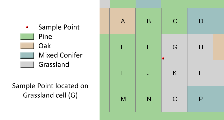
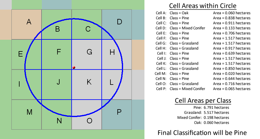
But the coordinates of that point are probably not known exactly — if a GPS receiver determined the location, the point may well have landed on the wrong cell of a perfectly correct classification. If you suspect significant locational uncertainty in your samples, a more conservative approach is to extract the majority value in a circular area around each point — a correction suggested by Dr. Russell Congalton for the original extension, and available in the Classification Accuracy tool as the circle-radius option (ties go to the value at the point). Note that the same point is classified differently using the circular area instead of the cell it happens to intersect:
As an aside: we strongly recommend reading past the “X-meter accuracy” blurb on the box your GPS came in. Most receivers define accuracy as a distance within which some percentage of fixes fall — and there is a very large difference between 50% of points within X meters (Circular Error Probable) and 95% of them.
Class proportions and error-adjusted areas
Everything above treats each sample point equally — which describes the sample. But the sample's class mix is rarely the landscape's class mix, and Card (1982)¶ showed that weighting the matrix cells by each class's true landscape proportion πi restores unbiased landscape-level accuracies, with variance formulas for both simple and stratified random sampling designs. The original kappa_stats extension implemented exactly this as its “weight analysis based on classification value landscape proportion” option.
Olofsson et al. (2014)¶ matured Card's weighting into the field's good-practice standard, with one decisive reframing: read in the other direction, the same machinery is an unbiased area estimator. The reference samples falling within each classified category tell you how that class's area truly divides among the ground classes — so the classification's own acreage figures can be corrected for misclassification, with standard errors.
A small example shows why this matters. Suppose a 10,000-ha classification shows 9,000 ha of forest and 1,000 ha of clearing, and the reference samples give a user's accuracy of 80% for classified clearing and 95% for classified forest — of the ground the classification calls clearing, 80% really is clearing; of the ground it calls forest, 95% really is forest. User's accuracy is the operative ingredient here, because the correction works from the classification's side: we stand on each classified category and ask what the reference samples found there. With only two classes, the 5% of classified forest that is not forest must be clearing, so the corrected clearing area is 1,000 × 0.80 + 9,000 × 0.05 = 1,250 ha — a full 25% more than the classification shows, because a small error rate applied to a large class moves more hectares than a large error rate applied to a small one. (Producer's accuracy — how much of the true clearing the classification managed to find — is what the correction produces, not what it consumes: with the corrected total in hand, the classification found 800 of the true 1,250 ha, a producer's accuracy of 64%.) No agreement statistic would ever reveal any of this; the area estimator is the tool that fixes the numbers you were going to quote from the classification. The Classification Accuracy tool measures the class proportions and the total classified area automatically from the classification dataset and reports each class's error-adjusted area in hectares with its standard error and confidence interval.
The modern statistics
- Weighted Kappa (Cohen 1968) serves ordinal classes — suitability ranks, cover classes — by weighting near-misses more gently than gross errors, with linear or quadratic weights.
- Gwet's AC1 (Gwet 2008)¶ is a chance-corrected agreement coefficient designed to resist the prevalence paradox: when one class dominates, Kappa can fall to embarrassingly low values even for classifications with excellent overall accuracy. AC1 models chance agreement differently and remains stable in imbalanced presence/absence designs.
- Quantity and allocation disagreement (Pontius and Millones 2011)¶ partition the total disagreement into two interpretable parts: how much of the error is in how much of each class the classification shows (quantity) versus where it put them (allocation) — a summary the critics of Kappa recommend in its place. Often the analyst or manager is more interested in learning what kind of repair the classification needs than in any single agreement number, and this partition answers exactly that. Consider the Pinaleños example from the tutorial. There, 39% of the samples disagree with the classification — the total disagreement, simply 1 − overall accuracy. Pontius and Millones split that 39% into two parts that sum exactly. Quantity disagreement (12%) is the share of samples that disagree simply because the classification draws too much of some classes and too little of others — its class totals do not match the reference totals, so some disagreement is unavoidable no matter where the classes are drawn. Allocation disagreement (27%) is the share that disagrees even though the totals could cover it — classes of roughly the right amounts drawn in the wrong places. Allocation errors come in pairs: a sample of Oak/Juniper mislabeled Mixed Conifer over here is balanced by a Mixed Conifer mislabeled Oak/Juniper over there, and swapping the two labels would fix both. The practical reading: re-tuning the classification's class totals — the cheap fix, a matter of adjusting thresholds — could at best erase the 12% quantity share, leaving 27% of the samples still wrong; repairing the 27% allocation share requires predictors that put the classes in the right places. That tells the analyst this classification needs spatially better information, not recalibrated proportions — a genuinely actionable conclusion. The quantity component is also the sample-side cousin of the error-adjusted areas: both notice that the classification's class totals are off; quantity/allocation tell you how much of your error budget that mismatch consumes, while the Olofsson estimators go on to fix the totals themselves.
- Bootstrap confidence intervals deserve more than the casual mention they usually get, so here is what the procedure actually does. The honest problem: a confidence interval requires knowing how much your statistic would wobble if you could repeat the whole field campaign many times — and you cannot. The bootstrap's answer is to let the sample stand in for the landscape: treat your n samples as if they were the population, and redraw n of them with replacement — so in each redraw some samples appear twice or three times and others not at all (about 37% sit out any given redraw). Each redraw is a plausible alternate version of your field campaign; recompute Kappa (or any statistic) on each of, say, 2,000 of them, and the spread of those 2,000 values is an honest estimate of the statistic's sampling distribution — no normality assumed. The middle 95% of them is the confidence interval, and unlike a ±Z interval it can never poke above 1 or below the statistic's real limits. The cost is only computation, which is no longer a cost; the benefit appears exactly where the normal approximation is doubtful — small samples, thin classes, or estimates near their ceiling.
The Kappa debate
A substantial modern literature argues against Kappa as a routine accuracy measure — most pointedly Pontius and Millones (2011, “Death to Kappa”)¶ and Foody (2020)¶. The complaints target the final summary statistic itself, not the analysis around it: Kappa measures agreement beyond chance rather than accuracy; its chance baseline is a poor model of how classifications actually err; and it is so sensitive to class prevalence that classifications with 95% overall accuracy can carry Kappa values anywhere from slightly below zero to 0.90 (Foody's own demonstration).
Rather than take that on faith, work through a small demonstration. Below are two error matrices of 200 samples each. In both classifications, every class is labeled with the same skill — and both have an overall accuracy of exactly 95%. The only thing that differs is how common the two classes are:
| Obs. A | Obs. B | |
|---|---|---|
| Pred. A | 95 | 5 |
| Pred. B | 5 | 95 |
| Obs. rare | Obs. common | |
|---|---|---|
| Pred. rare | 5 | 5 |
| Pred. common | 5 | 185 |
Same overall accuracy, yet Kappa falls from 0.90 to 0.47 — nearly halved — purely because one class became rare, which inflates the chance-agreement term. Now ask: which numbers actually tell you something you can act on? In Classification 2, the rare class's user's and producer's accuracies are both 5 / 10 = 50% — a coin flip. If that rare class is the wetland or the critical habitat your study cares about, the per-class table states the problem plainly, while the single Kappa of 0.47 only mutters something ambiguous: is this a mediocre classification, or a decent one applied to an imbalanced landscape? You cannot tell from Kappa alone — and that is the critics' entire point.
Hence what they recommend reporting instead: the full error matrix (which contains everything), overall accuracy with its interval, the per-class user's and producer's accuracies (which localize the problem), and the area-adjusted good-practice estimates (Olofsson et al. 2014; Stehman and Foody 2019¶ — which fix the acreage the errors distort), with McNemar's test as the recommended way to compare classifications evaluated on the same samples. Readers will notice that this is precisely the report the Classification Accuracy tool produces.
Kappa nonetheless keeps its adherents. It anchors the standard textbook treatment (Congalton and Green 1999) and decades of published accuracy statements that new work must be compared against — and even Foody grants it a legitimate remaining niche in assessing agreement among multiple interpreters, which is exactly the observer-comparison analysis these tools inherit from the original extension. For the prevalence paradox specifically, Gwet's AC1 is the robust alternative.
Case study — Mexican Jay distribution surfaces, Pinaleños Mountains, Arizona
A brief case study, based on research conducted by Wynne (2003)¶, illustrates how these statistics work together when neither model is statistically distinguishable from chance — a situation that may be familiar to anyone who models rare species. Two predictive habitat surfaces for the Mexican jay (Aphelocoma ultramarina) were compared: a classification-tree model built from a 1993–95 retrospective dataset, and a literature-based model built from published habitat accounts. Both models classify the same landscape into predicted habitat and predicted non-habitat, and both were assessed against the same field observation points:
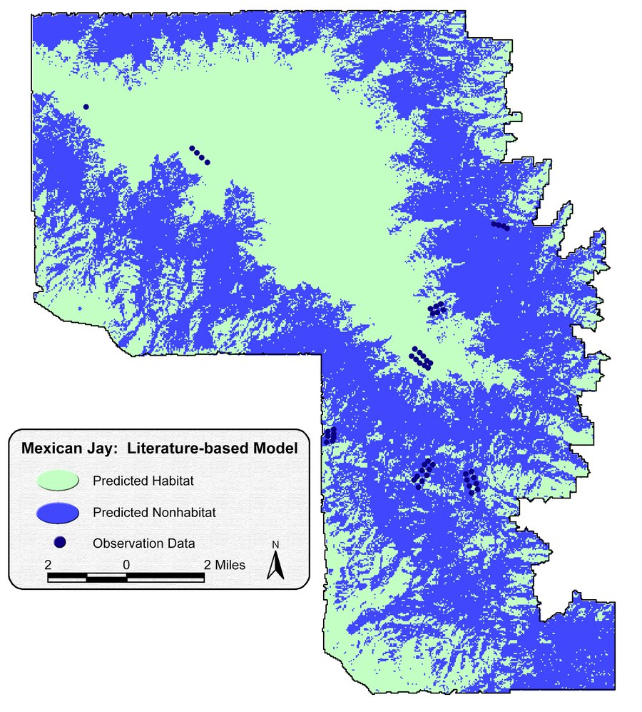
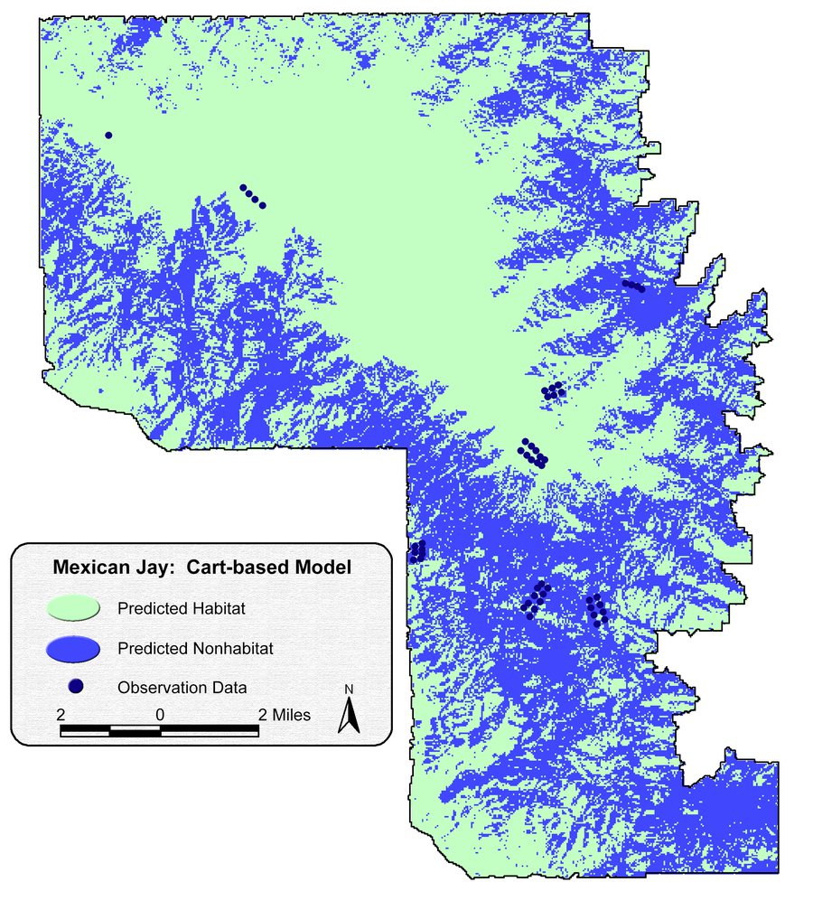
A statistical comparison suggested no significant difference between the two models (Z = 0.335, p = 0.369), and neither model's Kappa was significantly better than chance.
However, using a multi-criteria model selection process — highest overall accuracy, lowest misclassification rate, highest , highest sensitivity and specificity, highest predictive power, lowest commission and omission — the classification-tree model outperformed the literature-based model on nearly every criterion (overall accuracy 63.6% vs. 56.8%; = 0.22 vs. 0.136; higher predictive power for both presence and absence). The case study provides a tractable method for identifying the model with the highest potential performance even when statistical significance is lacking — often the honest situation with limited field data.
The same analysis through the modern report
The two error matrices from the reconstructed analysis (44 field observation points; 11 observed presences, 33 observed absences):
| Obs. habitat | Obs. nonhabitat | |
|---|---|---|
| Pred. habitat | 7 | 16 |
| Pred. nonhabitat | 4 | 17 |
| Obs. habitat | Obs. nonhabitat | |
|---|---|---|
| Pred. habitat | 8 | 12 |
| Pred. nonhabitat | 3 | 21 |
| Statistic | CART model | Literature model |
|---|---|---|
| Overall accuracy (95% CI) | 0.545 (0.389–0.696) | 0.659 (0.501–0.795) |
| No-information rate; P(accuracy > NIR) | 0.750; P = 0.999 | 0.750; P = 0.937 |
| Cohen's Kappa (95% CI); Z; P | 0.111 (−0.136–0.358); 0.88; 0.378 | 0.286 (0.024–0.547); 2.14; 0.032 |
| Gwet's AC1 (SE) | 0.136 (0.161) | 0.373 (0.149) |
| McNemar marginal symmetry | χ² = 6.05; P = 0.014 | χ² = 4.27; P = 0.039 |
| Pontius quantity / allocation | 0.273 / 0.182 | 0.205 / 0.136 |
| Habitat: user's / producer's accuracy | 0.304 / 0.636 | 0.400 / 0.727 |
| Habitat F1; negative predictive power | 0.412; 0.810 | 0.516; 0.875 |
| Error-adjusted habitat area (Olofsson) | 10,030 ± 2,803 ha (16,799 ha as drawn) |
— (needs the model raster's proportions; that surface is likewise lost to time) |
| Models compared (pairwise) | Z = 0.95, P = 0.341; common Kappa 0.193, P(equal) = 0.341 | |
Reading the table with the tools of this page in hand, four things stand out that the original overall-accuracy-and-Kappa summary could not show. First, neither model clears the no-information rate: with 33 of 44 observations being absences, always guessing “nonhabitat” scores 75%, a floor neither model's accuracy approaches — the rare-species prevalence problem in its purest form, and the reason the per-class rows matter more than the overall ones here. Second, both models fail the marginal-symmetry test in the same direction: each predicts roughly twice as much habitat as the observers found (23 and 20 predicted presences against 11 observed), a directional bias — though arguably the forgiving direction for a species of conservation concern, since habitat over-drawn invites a survey while habitat omitted invites a bulldozer. Third, the error-adjusted area quantifies that generosity for the CART surface: the reconstruction draws 16,799 ha of habitat, while the samples support an estimate of only about 10,030 ± 2,803 ha. And fourth, the punchline the original study reached by other means still stands: although the literature model's Kappa is individually distinguishable from chance here and the CART model's is not, the pairwise test cannot tell the two models apart (P = 0.341) — forty-four samples simply lack the power — so a defensible choice between them still rests on the multi-criteria comparison, exactly as Wynne concluded. The alert reader will notice that the bold now sweeps the literature model's column, where Wynne's 2003 table favored the CART model on nearly every criterion. We would not read too much into the reversal — a reconstructed surface, a different sample vintage, and only 44 points make the ranking itself delicate, which is precisely why the significance test declines to pick a winner — but it is a fair illustration of how the multi-criteria sweep works: line up every statistic, bold the better column, and let the preponderance speak, while holding the verdict as lightly as the sample size deserves.
References
- Agresti, A. 1990. Categorical Data Analysis. John Wiley and Sons, New York.
- Allouche, O., A. Tsoar, and R. Kadmon. 2006. Assessing the accuracy of species distribution models: prevalence, kappa and the true skill statistic (TSS). Journal of Applied Ecology 43:1223–1232. doi.org/10.1111/j.1365-2664.2006.01214.x
- Bowker, A. H. 1948. A test for symmetry in contingency tables. Journal of the American Statistical Association 43:572–574. doi.org/10.1080/01621459.1948.10483284
- Brodersen, K. H., C. S. Ong, K. E. Stephan, and J. M. Buhmann. 2010. The balanced accuracy and its posterior distribution. Proceedings of the 20th International Conference on Pattern Recognition, 3121–3124. doi.org/10.1109/ICPR.2010.764
- Card, D. H. 1982. Using known map category marginal frequencies to improve estimates of thematic map accuracy. Photogrammetric Engineering and Remote Sensing 48:431–439. ntrs.nasa.gov/citations/19820041921
- Cohen, J. 1960. A coefficient of agreement for nominal scales. Educational and Psychological Measurement 20:37–46.
- Cohen, J. 1968. Weighted kappa: nominal scale agreement with provision for scaled disagreement or partial credit. Psychological Bulletin 70:213–220.
- Congalton, R. G. 1991. A review of assessing the accuracy of classifications of remotely sensed data. Remote Sensing of Environment 37:35–46.
- Congalton, R. G., and K. Green. 1999. Assessing the Accuracy of Remotely Sensed Data: Principles and Practices. Lewis Publishers.
- Congalton, R. G., and R. A. Mead. 1983. A quantitative method to test for consistency and correctness in photointerpretation. Photogrammetric Engineering and Remote Sensing 49:69–74.
- Fielding, A. H., and J. F. Bell. 1997. A review of methods for the assessment of prediction errors in conservation presence/absence models. Environmental Conservation 24:38–49.
- Fleiss, J. L. 1981. Statistical Methods for Rates and Proportions, 2nd ed. John Wiley and Sons, New York.
- Fleiss, J. L., J. Cohen, and B. S. Everitt. 1969. Large sample standard errors of kappa and weighted kappa. Psychological Bulletin 72:323–327.
- Foody, G. M. 2004. Thematic map comparison: evaluating the statistical significance of differences in classification accuracy. Photogrammetric Engineering & Remote Sensing 70:627–633. doi.org/10.14358/PERS.70.5.627
- Foody, G. M. 2020. Explaining the unsuitability of the kappa coefficient in the assessment and comparison of the accuracy of thematic maps obtained by image classification. Remote Sensing of Environment 239:111630. doi.org/10.1016/j.rse.2019.111630
- Gwet, K. L. 2008. Computing inter-rater reliability and its variance in the presence of high agreement. British Journal of Mathematical and Statistical Psychology 61:29–48. doi.org/10.1348/000711006X126600
- Jenness, J. and J. J. Wynne. 2007. Cohen's Kappa and classification table metrics 2.1a (kappa_stats.avx). Jenness Enterprises. jennessent.com/arcview/kappa_stats.htm
- Kuhn, M. 2008. Building predictive models in R using the caret package. Journal of Statistical Software 28(5):1–26. doi.org/10.18637/jss.v028.i05
- McNemar, Q. 1947. Note on the sampling error of the difference between correlated proportions or percentages. Psychometrika 12:153–157. doi.org/10.1007/BF02295996
- Olofsson, P., G. M. Foody, M. Herold, S. V. Stehman, C. E. Woodcock, and M. A. Wulder. 2014. Good practices for estimating area and assessing accuracy of land change. Remote Sensing of Environment 148:42–57. doi.org/10.1016/j.rse.2014.02.015
- Pontius, R. G., Jr., and M. Millones. 2011. Death to Kappa: birth of quantity disagreement and allocation disagreement for accuracy assessment. International Journal of Remote Sensing 32:4407–4429. doi.org/10.1080/01431161.2011.552923
- Sokolova, M., and G. Lapalme. 2009. A systematic analysis of performance measures for classification tasks. Information Processing and Management 45:427–437. doi.org/10.1016/j.ipm.2009.03.002
- Stehman, S. V., and G. M. Foody. 2019. Key issues in rigorous accuracy assessment of land cover products. Remote Sensing of Environment 231:111199. doi.org/10.1016/j.rse.2019.05.018
- Story, M., and R. G. Congalton. 1986. Accuracy assessment: a user's perspective. Photogrammetric Engineering and Remote Sensing 52:397–399.
- Van Rijsbergen, C. J. 1979. Information Retrieval, 2nd ed. Butterworths, London.
- Wynne, J. J. 2003. Landscape-scale modeling of vegetation land cover and songbird habitat, Pinaleños Mountains, Arizona. M.S. thesis, Northern Arizona University, Flagstaff.
Related pages
- Footnotes — what the cited authors actually said — verbatim supporting statements, with page numbers, for the citations on this page.
- Classification Accuracy (Kappa) — the tool that computes everything described here.
- Kappa analysis tutorial — a complete worked assessment on the Pinaleños dataset.