

Estimate Sample Size
Summary
Estimates the reference sample size needed for a statistically defensible accuracy assessment — the question to answer before the field work begins. Pick one of four methods, ordered by how much you know: Congalton and Green's multinomial approach (after Tortora 1978) as the worst case with no class proportions known, refined by the largest class proportion, or from per-class proportions with individual precision requirements — each with the optional finite population correction — or the Olofsson et al. (2014) sample size for a target standard error of overall accuracy. Returns the recommended size as a derived output for ModelBuilder.
A port of the classic kappa_stats extension's Sample Size tool, and it reproduces that extension's published example table to the sample. There is no equivalent among the standard ArcGIS Pro geoprocessing tools.
Usage
Answers “how many reference samples do I need?” while the answer can still shape the field season. Too few samples leave the accuracy estimates so wide that nothing can be concluded from them; far too many spends field time that the statistics never repay. Each of the four methods turns what you already know about the classification into a defensible number, and the less you know, the larger — and safer — the answer.
The multinomial methods (Congalton and Green, after Tortora 1978)
An accuracy assessment is a multinomial problem: every reference sample lands in exactly one class, and we want every class's estimate to hold at the stated confidence simultaneously. Tortora's (1978) solution, adopted by Congalton and Green as their recommended practice¶, sizes the sample from the binding class:
where p is a class proportion, b is the desired precision (the acceptable half-width of the accuracy estimate, as a proportion), and B is a chi-square critical value with one degree of freedom carrying a Bonferroni share of the alpha — α/k apiece across the k classes, which is how the simultaneous guarantee is bought. More classes mean a larger B, and therefore more samples. The three multinomial methods differ only in what they feed this formula:
- Worst case (no class proportions known). Enter only the number of classes, the confidence level, and the desired precision. A class at exactly 50% — the largest possible variance — is assumed, giving the largest safe answer.
- Largest class proportion known. Also enter the largest class's proportion of the classification. Since the proportions sum to 100%, the largest class is always the one closest to 50%, and its variance governs the whole design; the farther it sits from 50%, the more the estimate tightens below the worst case.
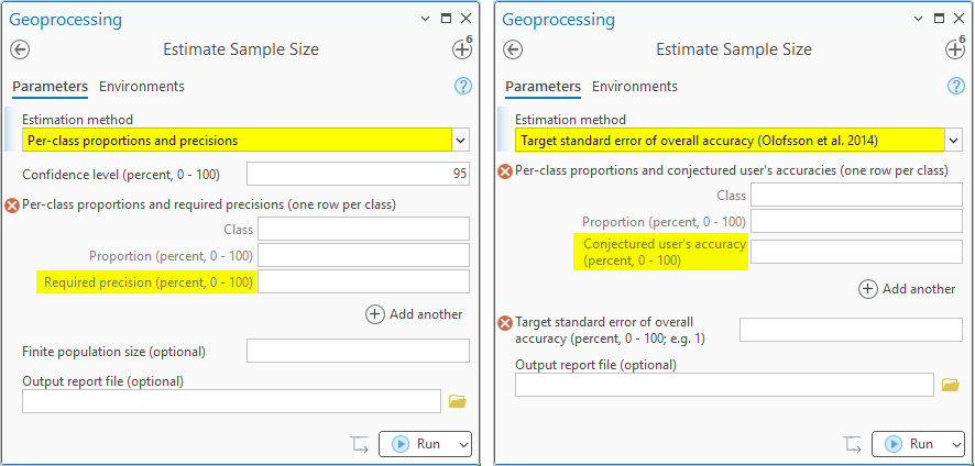
- Per-class proportions and precisions. Enter one row per class: its proportion and its own required precision — how tightly you need that particular class's accuracy estimate pinned down. The formula runs once per class and the most demanding class governs; tightening the precision on one critical class raises the whole total. The class count comes from the rows you enter.
All three accept the optional finite population correction — sampling theory's standard allowance for drawing from a limited universe (Thompson 2002)¶ — for when only a limited number of samples exists at all: a fixed frame of N photo-interpretation plots, for example:
The required sample shrinks as n approaches N, and the tool's derived output carries the correction whenever a population is given. (This is the finite-population variance carried through the sample-size algebra — algebraically identical to Tortora's equation 2.9.)
Here is the method at work on the tutorial's four-class Pinaleños classification, whose largest class (Oak/Juniper) covers 43% of the landscape, at 95% confidence and 10% precision:
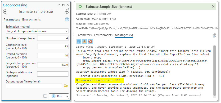
The answer is 153 samples — against 156 had we known nothing about the proportions at all. The gap is small because 43% sits so near the worst case; a classification dominated by one class at 80% would tighten much further, to 100 samples for the same confidence and precision.
Planning for area-weighted assessments (Olofsson et al. 2014)
The fourth method is the planning route for modern area-weighted assessments — the kind whose goal is not just an accuracy figure but error-adjusted class areas with confidence intervals (the Olofsson block of the Classification Accuracy (Kappa) report). Choose a target standard error of overall accuracy and enter one row per class: its proportion and a conjectured user's accuracy — your best planning guess of how accurate the classification actually is for that class. If you expect 19 out of 20 cells labeled as a class to be correct, enter 95; if you expect only half of them to be, enter 50. Equation 13 of Olofsson et al. (2014)¶ then gives the total:
where Wi are the class proportions, S(Ô) is the target standard error, and each class's standard deviation comes from its conjectured user's accuracy Ui.
Notice what the formula implies: guesses nearer 50% carry more variance and demand more samples, so an honest or slightly pessimistic guess is the conservative choice. On the tutorial's classification, pinning overall accuracy to a ±1-percentage- point standard error takes about 774 samples with optimistic guesses (85–95%) — and climbs toward 2,500 as the guesses fall to 50%. An inaccurate classification needs far more samples to pin down, which is a planning lesson worth absorbing before the trucks are loaded. Olofsson et al. also recommend allocating 50–100 samples to rare-but-important classes and distributing the rest proportionally.
Rules of thumb
Congalton and Green temper the formulas with field-tested practice: a minimum of about 50 samples per class, rising to 75–100 per class when the classification distinguishes many classes (more than about 12), and never leave a class unsampled — accuracy cannot be estimated for a class that was never checked. The tool's report closes with this reminder alongside the recommended total.
In R
There is no standard packaged R function for the multinomial sample size — but the arithmetic is a handful of lines, and the tool writes them for you: every report closes with an R cross-check of the very estimate it just made, your numbers baked in and the expected answer in the trailing comment, ready to copy and paste straight into R. The block below checks the whole ladder at once on the tutorial's numbers — exactly the cross-check we keep in this suite's permanent test set:
B <- qchisq(1 - (1 - 0.95) / 4, df = 1)  # Bonferroni share of alpha, k = 4
ceiling(B * 0.50 * 0.50 / 0.10^2)        # worst case                  -> 156
ceiling(B * 0.43 * 0.57 / 0.10^2)        # largest class at 43%        -> 153
n <- B * 0.25 / 0.10^2                   # finite population, N = 10,000:
ceiling(n / (1 + (n - 1) / 10000))       # worst case with the FPC     -> 154

W <- c(0.4299, 0.3572, 0.1315, 0.0813)   # class proportions
U <- c(0.90, 0.95, 0.85, 0.90)           # conjectured user's accuracies
ceiling((sum(W * sqrt(U * (1 - U))) / 0.01)^2)  # 1% target SE         -> 774
ModelBuilder
The tool offers two outputs to a model: the optional text report, and the derived Recommended sample size — carrying the finite population correction when a population was given — ready to feed the number-of-points parameter of the Random Point Generator or the sample size of Select Random Records, so nothing is retyped between planning the design and drawing it:
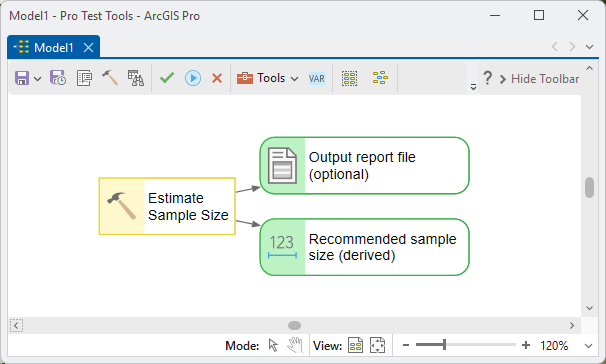
The tutorial's Step 1 shows this same output chained straight into the Random Point Generator.
Parameters
| Label | Explanation | Data type |
|---|---|---|
| Estimation methodRequired · method | Which of the four estimators to run; only that method's parameters stay enabled. Worst case: nothing known beyond the class count — the largest safe answer. Largest class proportion known: tightens the worst case using the largest class's proportion. Per-class proportions and precisions: the most demanding class governs. Target standard error (Olofsson et al. 2014): the planning route for area-weighted assessments, from conjectured user's accuracies. | String |
| Number of map classesOptional · n_classes | How many classes the classification distinguishes. The confidence level is Bonferroni-shared across them, so more classes require more samples. For the per-class methods the count comes from the per-class rows instead. | Long |
| Confidence level (percent, 0 - 100)Optional · confidence | The probability the sample will support statistically valid accuracy conclusions (default 95). | Double |
| Desired precision (percent, 0 - 100)Optional · precision | The acceptable half-width of the accuracy estimates (default 10). Tighter precision raises the sample size quadratically. | Double |
| Largest class proportion (percent, 0 - 100)Optional · max_prop | The proportion of the classification covered by its largest class — always the class closest to 50%, whose variance governs the sample size. Read it from the classified raster's attribute table or the polygon areas. | Double |
| Per-class proportions and required precisionsOptional · class_table | One row per class: its proportion (percent) and its required precision (percent) — how tightly that class's accuracy estimate must be pinned down. A statement about the quality of the estimate you want, not about how accurate you expect the classification to be. The most demanding class governs. | Value Table |
| Per-class proportions and conjectured user's accuraciesOptional · ua_table | One row per class: its proportion (percent) and its conjectured user's accuracy (percent) — your best planning guess of how accurate the classification actually is for that class. Guesses nearer 50% are conservative, so guess low when unsure. | Value Table |
| Finite population sizeOptional · population | The total number of possible samples (a fixed plot frame). The finite population correction shrinks the required n, and the derived recommended size carries it. | Double |
| Target standard error of overall accuracy (percent; e.g. 1)Optional · target_se | The target standard error for overall accuracy, in percentage points — 1 means the estimate should carry a standard error of about one percentage point. (The Classification Accuracy report prints its achieved standard errors as proportions; 1% = 0.01.) | Double |
| Output report fileOptional · out_report | A text file holding the sample-size report (it also prints in the messages). | File |
| Recommended sample sizeDerived · out_n | The recommended sample size for the chosen method, with the finite population correction applied when a population was given — connect it to the Random Point Generator or Select Random Records in ModelBuilder. | Long |
Python
The classic extension manual's published scenario: four classes at 95% confidence and 10% precision, the largest class at 36.7%, over a 10,000-plot frame:
import arcpy
arcpy.ImportToolbox(r"C:\path\to\JennessEnterprisesTools.pyt")  # your install path
result = arcpy.jenness.AccuracySampleSize(
    method="Largest class proportion known",
    n_classes=4, confidence=95, precision=10,
    max_prop=36.7, population=10000)
print(result.getOutput(1))  # the recommended sample size -> 143
Recommended citation
Credits and references
By Jeff Jenness, Jenness Enterprises (www.jennessent.com), and J. J. Wynne, Department of Biological Sciences and Center for Adaptive Western Landscapes, Northern Arizona University. A port of the Sample Size tool of: Jenness, J. and J. J. Wynne (2007), Cohen's Kappa and classification table metrics 2.1a (kappa_stats.avx), Jenness Enterprises.
- Congalton, R. G., and K. Green. 1999. Assessing the Accuracy of Remotely Sensed Data: Principles and Practices. Lewis Publishers, Boca Raton, Florida.
- Olofsson, P., G. M. Foody, M. Herold, S. V. Stehman, C. E. Woodcock, and M. A. Wulder. 2014. Good practices for estimating area and assessing accuracy of land change. Remote Sensing of Environment 148:42–57. doi.org/10.1016/j.rse.2014.02.015
- Thompson, S. K. 2002. Sampling, 2nd ed. John Wiley and Sons, New York.
- Tortora, R. D. 1978. A note on sample size estimation for multinomial populations. The American Statistician 32:100–102. doi.org/10.1080/00031305.1978.10479265
Licensing information
Works at every ArcGIS Pro license level (Basic, Standard, Advanced). No extension licenses are required.
Related tools and pages
- Random Point Generator — draws the design this tool sizes, stratified by the classification's classes.
- Select Random Records — selects the sample from an existing frame of candidate plots.
- Classification Accuracy (Kappa) — runs the assessment the samples feed.
- Compare Accuracy Analyses — tests whether two or more finished assessments differ.
- About Kappa and classification accuracy analysis — designing the assessment, from classification scheme to sample size.
- Kappa analysis tutorial — this tool demonstrated on the Pinaleños classification (Step 1).
- Footnotes — what the cited authors actually said, verbatim.