

Estimated Shortest Path through Points
Summary
Orders a set of points into a short travel route — a survey route you can load straight into a GPS. Three route types: a simple shortest path (the route starts and ends at whichever two of your points give the shortest total), a round trip from a single start/end point (for example, where you left the truck), or a route from a fixed start point to a fixed end point. The tool writes the route polyline and, optionally, a copy of your points numbered in visit order, plus derived stop-count and route-length values for ModelBuilder.
Legs are straight lines between locations, not road-network routes — exactly what cross-country fieldwork wants, and a different problem from the one Esri's Network Analyst solves (see Licensing).
The question every sampling design leaves behind
You have generated your sample locations — now you have to go stand on every one of them. The Random Point Generator, the Random Sample Array Generator, Repeating Shapes, and the Spatially Balanced Sample (GRTS) tool are all careful to place sites without regard to your convenience — that indifference is precisely what makes the samples defensible — and so the very first practical question after the design is drawn is: in what order should I visit these points, so I spend my field season surveying instead of walking?
The order matters more than intuition suggests. On the Random Sample Array Generator page we routed the same 150 stations two ways and the difference was 22.4 km against 40.4 km — nearly a factor of two, purely from visiting order and design. This tool finds a good order automatically, for any point feature class — its natural companions are the four generators above, but any points work, and a layer's selection is honored.
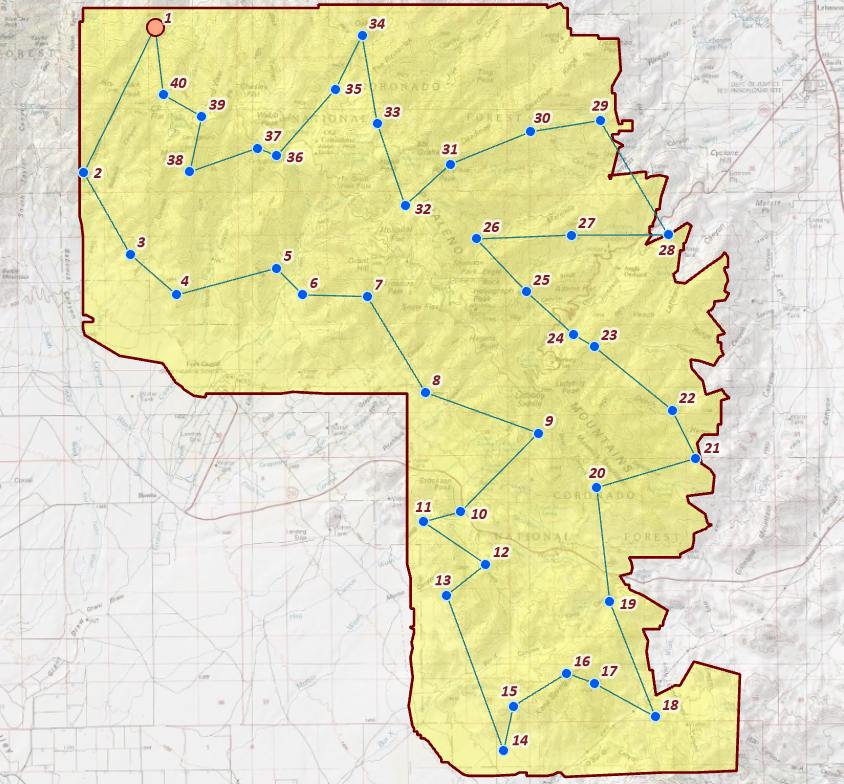
Three route types
Simple Shortest Path finds the shortest open path through all the points, starting and ending at whichever two of your own points give the shortest total. Use it when you simply want the points ordered efficiently and do not care where the route begins — and note that it costs nothing extra: the solver treats the two endpoints as one more thing to optimize.
Start and End at Same Point makes a round trip: give a single point — for example, where you left the truck — and the route leaves it, visits every point, and returns to it. The trip in the figure above is this mode.
Start and End at Different Specified Points runs from a fixed start to a fixed end — a trailhead to a pickup spot, a put-in to a take-out.
For the last two modes, each start/end feature class must supply exactly one point: either a feature class holding a single point, or one selected point on a larger layer. If the layer supplies more than one, the tool stops with a plain message rather than guessing which point you meant.
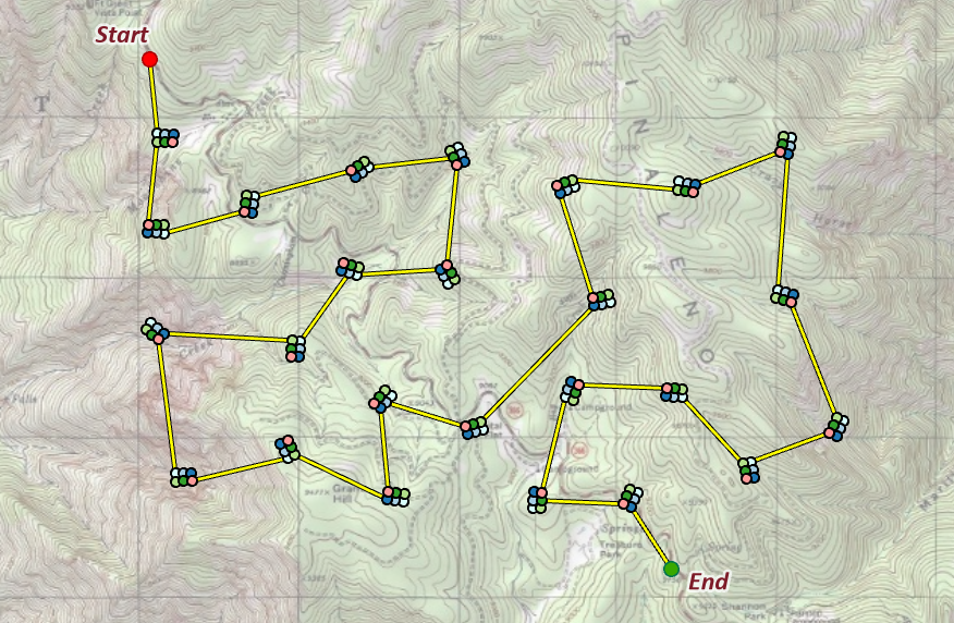
How the tool estimates the shortest path
Finding the truly shortest route through many points is the classic traveling-salesperson problem, and exact answers are computationally out of reach beyond a few dozen points — which is why the word Estimated is in this tool's name rather than buried in a footnote. The tool uses a careful, well-studied heuristic recipe:
- Build candidate routes two classic ways — nearest-neighbor (always walk to the closest unvisited point) and cheapest-insertion (grow the route by adding whichever point fits in cheapest) — plus a few randomized starting orders.
- Polish every candidate with two refinement moves, applied over and over until neither finds anything: 2-opt (Croes 1958) uncrosses the route wherever reversing a stretch shortens it, and Or-opt relocates short runs of three, two, then one consecutive stops to better positions, forward or reversed (the longest-first order that Babin, Deneault, and Laporte 2007 measured best).
- Keep the shortest. The same inputs always produce the same route — there is no hidden randomness to make a rerun disagree with your map.
More powerful methods exist: the celebrated variable-depth search of Lin and Kernighan (1973) and its descendants can edge within about a percent of the true optimum. But they are famously delicate to implement correctly, and a subtly wrong route solver fails silently — it hands you a confident-looking route that is quietly longer than it should be. This tool deliberately stays with the simpler, verifiable move family, the same trade Laporte's group recommends for practical use; the price, in testing, is a few percent at most on realistic problems.
Speed and the practical ceiling. A thousand points solve in about a second. Effort grows with the square of the point count, and the practical ceiling is roughly 8,000 points — beyond that the tool stops with a friendly suggestion to split the survey into regions and route each on its own (which is also better field logistics). Points in latitude–longitude are handled in an automatic equal-area working projection, and route lengths are reported as true geodesic distances either way.
How we checked our work
A heuristic that promises “within a few percent of optimal” should have to prove it. The honest way to prove it is to compare against the true optimum — not another heuristic, not a guess, but the actual best possible route — and the only way to know the true optimum for certain is brute force: try every conceivable order of stops, measure each one, and keep the shortest. That is wildly impractical for a real survey — a mere 20 stops have more possible orders (about 2.4 quintillion) than seconds have ticked by since the Big Bang — but it is entirely practical for a small problem, and a heuristic that is any good should match brute force whenever brute force is affordable.
So the tool's permanent test suite does exactly that, on problems just large enough to be interesting and just small enough to check exhaustively: seven stops between a fixed start and end (5,040 possible orders — that's 7 factorial, small enough for a laptop to check every single one in a blink) for the open-path modes, and eight stops arranged in a loop for the round trip mode. Thirty such problems were generated at random — twenty open paths, ten round trips — brute force computed the genuinely shortest route for each, and the tool's heuristic was run on the identical points. In every one of the thirty comparisons, the heuristic's route matched the brute-force optimum exactly — not close, not “within a few percent,” but the same route, to the meter.
The suite also checks a handful of problems simple enough that you can see the right answer without any computer at all, which catches a different kind of bug — not “is this route a little too long” but “is the logic actually correct.” A row of points strung out along a line must be visited in order along the line; any zigzag would obviously backtrack and waste distance. A round trip that visits the four corners of a square must trace the square's perimeter exactly — any other order revisits a side. And when both ends of the route are left for the solver to choose (the Simple Shortest Path mode), points arranged in a line must have the route begin and end at the two far ends of that line — starting anywhere in the middle would force a wasted trip back past already-visited points. The suite also confirms the tool is deterministic: given the same points and the same settings, two separate runs produce the exact same route, not just a similar one — useful to know if you ever need to explain to a reviewer why your GPS track matches your map exactly. And a timing check confirms that a thousand-point problem — far more stops than most surveys will ever have — still solves in about a second, so the tool stays practical at real-world scale.
None of this guarantees exact optimality on your own 500-station survey — no fast method can promise that, and this tool is honest about being an estimate rather than a proof. What it does mean is that the machinery has been shown, repeatedly and rigorously, to find the true best answer whenever we can actually afford to check one — which is the strongest evidence available that it is finding very good answers when we can't.
What you get
The route polyline carries Route_Type (which of the three modes drew it), N_Stops, Length_km, and Length_mi — the lengths computed geodesically. Ask for the optional points numbered in visit order and you also get a copy of your points with:
- Visit_Order — 1, 2, 3, … in route order. Label the points with it and the map reads like an itinerary (the round-trip figure above is labeled exactly this way).
- Src_FID — the source point's Object ID, so every stop joins back to your original attributes.
- Leg_km — the length of the leg leaving each stop, handy for planning water, daylight, and rendezvous times. The last stop of an open path carries 0; on a round trip the final leg runs back to the start point.
A tour of the dialog
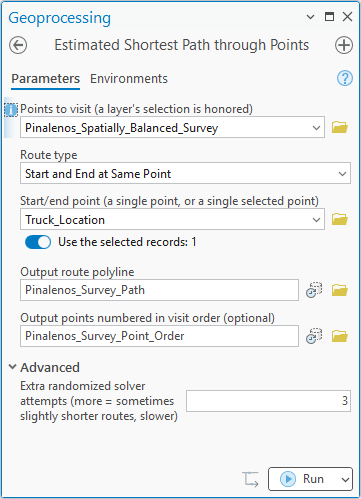
The dialog stays small: the points, the route type, the start/end point classes the chosen type reveals, and the outputs. Note in the figure that the start/end point is supplied by a layer with one selected record — the “single point or single selected point” rule in action. Under Advanced, extra randomized solver attempts re-polish from additional shuffled starting orders and keep the best; the default of 3 is a good balance, and the result is deterministic either way.
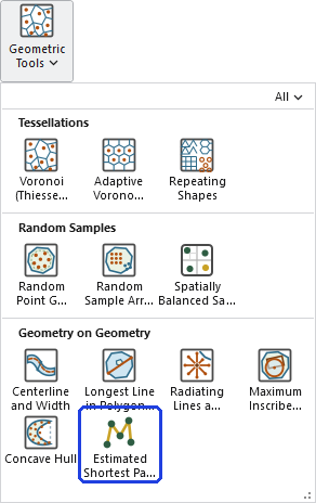
ModelBuilder
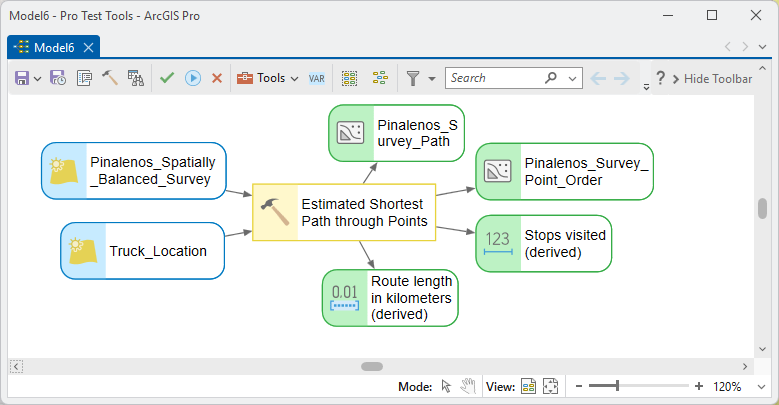
The tool offers a model the route polyline, the optional visit-ordered points, and two derived scalars — stops visited and route length in kilometers — so a model can chain straight from design to logistics: draw the sample with the Spatially Balanced Sample (GRTS) tool or the Random Point Generator, route it here, and hand the length to whatever comes next (per-day planning, cost estimates, a report).
Parameters
| Label | Explanation | Data type |
|---|---|---|
| Points to visitRequired · in_points | The points to route through — typically sample locations from this suite's point generators, but any point feature class or layer works. A selection is honored; multipoints are exploded. | Feature Layer |
| Route typeRequired · mode | Simple Shortest Path (endpoints chosen from your points), Start and End at Same Point (a round trip), or Start and End at Different Specified Points. | String |
| Start/end pointOptional · loop_point | Round trips only: the point the route leaves from and returns to — for example, where you left the truck. A single-point feature class, or one selected point on a larger layer. | Feature Layer |
| Start pointOptional · start_point | Fixed start/end routes only: where the route begins. Single point or single selected point. | Feature Layer |
| End pointOptional · end_point | Fixed start/end routes only: where the route ends. Single point or single selected point. | Feature Layer |
| Output route polylineRequired · out_route | The route as one polyline visiting every point: Route_Type, N_Stops, Length_km, Length_mi (geodesic). A suggested name is filled in from the input. | Feature Class |
| Output points numbered in visit orderOptional · out_points | A copy of the points with Visit_Order, Src_FID, and Leg_km. | Feature Class |
| Extra randomized solver attemptsOptional · attempts | Advanced: additional shuffled starting orders to polish beyond the standard constructions (default 3). More attempts occasionally shave a little length at a proportional cost in time; deterministic either way. | Long |
| Stops visitedDerived · out_n | The number of points visited, for ModelBuilder chains. | Long |
| Route length in kilometersDerived · out_length_km | The route's total geodesic length, for ModelBuilder chains. | Double |
Python
A round trip through survey stations from the parking spot, with the visit-ordered points saved alongside the route:
import arcpy
arcpy.ImportToolbox(r"C:\path\to\JennessEnterprisesTools.pyt")  # your install path
# mode options (matching is by prefix):
#   "Simple Shortest Path"
#   "Start and End at Same Point"
#   "Start and End at Different Specified Points"
result = arcpy.jenness.EstimatedShortestPath(
    in_points=r"D:\data\study.gdb\stations",
    mode="Start and End at Same Point",
    loop_point=r"D:\data\study.gdb\parking",
    out_route=r"D:\data\study.gdb\stations_Route",
    out_points=r"D:\data\study.gdb\stations_Visit_Order")
print(result.getOutput(2))  # stops visited
print(result.getOutput(3))  # route length, km
Recommended citation
Credits and references
By Jeff Jenness, Jenness Enterprises (www.jennessent.com). Route refinement after the classic 2-opt of Croes (1958) and Or-opt segment relocation as described by Babin, Deneault, and Laporte (2007); the Or-opt move family is named for Ilhan Or's 1976 Northwestern dissertation, which we were unable to access. The variable-depth alternative discussed above is Lin and Kernighan (1973).
- Babin, G., S. Deneault, and G. Laporte. 2007. Improvements to the Or-opt heuristic for the symmetric travelling salesman problem. Journal of the Operational Research Society 58(3):402–407. doi.org/10.1057/palgrave.jors.2602160
- Croes, G. A. 1958. A method for solving traveling-salesman problems. Operations Research 6(6):791–812. doi.org/10.1287/opre.6.6.791
- Lin, S., and B. W. Kernighan. 1973. An effective heuristic algorithm for the traveling-salesman problem. Operations Research 21(2):498–516. doi.org/10.1287/opre.21.2.498
Licensing information
Works at every ArcGIS Pro license level (Basic, Standard, Advanced). No extension licenses are required. Note the division of labor with Esri's tools: Network Analyst's Route solves a different problem — travel along a road network, which requires both the extension and a network dataset. This tool routes between locations as the crow flies, which is what cross-country fieldwork wants; and even when you will drive between points, the visiting order it finds is usually an excellent order to feed a road-based navigator.
Related tools and pages
- Spatially Balanced Sample (GRTS) — the survey design routed in the figures above.
- Random Point Generator — random designs with spacing and boundary constraints; route the result here.
- Random Sample Array Generator — cluster arrays whose field economics this tool's routing completes; its page carries the 22.4-vs-40.4 km comparison.
- Repeating Shapes — systematic designs; their regularity routes especially well.