

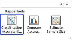
Classification Accuracy (Kappa)
Summary
Assesses the accuracy of a categorical classification or model against reference (field-verified) classes: the error matrix, Cohen's Kappa with variance, Z test and confidence interval, weighted kappa, per-class conditional kappa, user's and producer's accuracies, the sensitivity/specificity family, F1, Gwet's AC1, Pontius–Millones disagreement, and the Olofsson et al. (2014) area-weighted accuracies and error-adjusted area estimates with confidence intervals. Values come from attribute fields or are extracted from classified rasters or polygon feature classes, optionally as the majority in a circle around each sample (locational uncertainty). The report ends with a ready-to-run R snippet reproducing the analysis.
A modernized port of Jenness and Wynne's classic Kappa analysis extension for ArcView 3.x, validated against R's reference packages. Unlike Esri's Compute Confusion Matrix — which requires Spatial Analyst or Image Analyst, is welded to the Accuracy Assessment Points schema, and reports no variances, intervals, tests or area estimates — this tool runs at every license level on any categorical pairing.
Usage
Assesses how well a categorical classification or predictive model matches reality: habitat suitability classes against field surveys, a vegetation classification against photo-interpreted plots, a land-cover dataset against reference imagery.
Inputs
The sample points (or table) hold the reference locations. The classification (predicted) classes and the observed (reference) classes each come from either an attribute field of the sample points or a classified dataset — a raster, or a polygon feature class with a class field, chosen from the map's layers or browsed from disk — extracted at each sample point. For rasters, the class field can name a raster attribute-table field (typically the class-name field), so extracted classes match a reference field that stores names rather than cell codes; blank uses the raw cell values.
The two sides' class vocabularies must match (names to names, or codes to codes), or every sample counts as disagreement. Selections are honored. Samples that cannot contribute — a NoData cell under the point, or a null value in a class field — are left out of the analysis, and the report prints how many were left out and why, so missing samples never disappear silently.
Locational uncertainty
If sample coordinates carry GPS error, a point can land on the wrong cell of a correct classification. The optional circle radius replaces the value-at-point with the majority value in a circle around each sample (ties go to the value at the point) — a correction suggested by Dr. Congalton. It applies to layer-extracted values only.
The classic statistics
- The error matrix, with overall accuracy and its exact binomial (Clopper–Pearson) confidence interval, the no-information rate test — the accuracy you could get by ignoring the samples entirely and always guessing the commonest reference class; a defensible classification should beat it convincingly, and the report tests whether yours does — and McNemar's marginal-symmetry test.
- Per-class user's accuracy (how reliable is the classification where it claims class X) and producer's accuracy (how much of the real class X did the classification find).
- Cohen's Kappa — agreement corrected for chance — with its delta-method variance (Fleiss, Cohen and Everitt 1969)¶, Z test against chance, and confidence interval, with the honest Chebyshev worst-case coverage note when normality is in doubt.
- Per-class conditional kappa with standard errors.
- The full 2×2 diagnostic family per class: sensitivity, specificity, omission and commission error, positive and negative predictive power, with weighted overall averages and the presence/absence guidance for two-class models.
The modern statistics
- Weighted kappa (Cohen 1968)¶ for ordinal classes — habitat suitability ranks, cover classes — with linear or quadratic weights, so near-misses count more than gross errors.
- F1 per class (the harmonic mean of user's and producer's
accuracy; also the Dice coefficient) and macro-F1 — the score the
species-distribution-modeling and machine-learning literature reports
— plus per-class prevalence, detection rate, detection
prevalence and balanced accuracy, so the report reads line-for-line
against R's
caret::confusionMatrixoutput. - Gwet's AC1 (Gwet 2008), a chance-corrected agreement robust to the prevalence paradox that deflates kappa in imbalanced presence/absence designs.
- Pontius–Millones quantity and allocation disagreement (Pontius and Millones 2011): how much of the error is in how much of each class versus where it was put — the field's recommended replacement summary (see The kappa debate below).
- Optional bootstrap percentile confidence intervals for kappa and overall accuracy (seeded, reproducible) — the modern answer where the normal approximation is doubtful. Each replicate redraws the full sample count with replacement from the original samples and recomputes the statistics; 1,000 to 2,000 replicates is the usual choice. As a rule of thumb the normal approximation is doubtful with fewer than roughly 100–200 samples in total, fewer than about 30–50 in any one class (Congalton and Green's design guideline is 50 per class), or an accuracy or kappa near its upper limit.
Area-weighted estimates and error-adjusted areas
Check Weight the analysis by map class proportions to add stratified overall/user's/producer's accuracies with standard errors, along with a powerful and modern application of the error matrix: error-adjusted area estimates, which combine the predicted classification dataset with the field observations at the sample points to estimate the true area of the landscape in each category, with confidence intervals (“the classification says 12,000 ha of aspen; the unbiased estimate is 9,400 ± 1,100 ha”).
The lineage of this option runs from Card (1982) to Olofsson et al.'s (2014) good-practice standard, which reframed the same weighting as an unbiased area estimator — the full story, with a worked example of why a small error rate in a large class can move more hectares than a large error rate in a small one, is told in About Kappa analysis.
Class proportions come automatically from the classification (predicted) dataset (with true areas calculated using geodesic methods for polygons, and latitude-corrected cell areas for geographic rasters) or can be typed in. The total classified area is measured from the same dataset automatically — the analyzed classes only, NoData excluded; for a geographic raster read through an attribute-table class field it is estimated from the cell area at the raster's central latitude — so the error-adjusted areas are reported in hectares automatically. If you have alternate information about the size of the study area (in hectares), you have the option to manually override the auto-calculated area by typing the area into the total-area parameter. This might happen if you have an official record of the map area, if you are entering class proportions typed by hand, or when the classes come from table fields alone and no raster or polygon dataset is available to calculate area from.
The kappa debate, in brief
A substantial modern literature argues against kappa as a routine accuracy measure (Pontius and Millones 2011, “Death to Kappa”; Foody 2020) — while what the critics recommend reporting instead is exactly what this tool produces: the full error matrix, overall accuracy, per-class user's and producer's accuracies, the area-adjusted good-practice estimates, and McNemar's test for same-sample comparisons. Report the matrix and the accuracies as the critics ask, and quote kappa knowingly — for comparability with the literature and for observer-agreement questions — rather than as the sole headline figure. The full discussion, including where kappa retains legitimate uses, is in About Kappa analysis.
Comparing analyses
An analysis field splits the samples — per observer, per model, per year — into separate analyses that are compared automatically: pairwise Z tests and the Fleiss (1981)¶ common-kappa chi-square test. The Compare Accuracy Analyses tool does the same from typed kappa/variance pairs.
The same analysis in R
Every statistic here has a reference implementation in R, several
maintained by the method authors themselves:
psych::cohen.kappa (kappa and its Fleiss-Cohen-Everitt
variance), caret::confusionMatrix (the per-class suite),
yardstick::kap (weighted kappa),
mapaccuracy::olofsson (the Olofsson estimators),
diffeR (Pontius's own package for quantity/allocation), and
irrCAC (Gwet's own package for AC1). This tool's algorithms
are validated against all of them to close to machine precision, and
every report ends with a ready-to-run R snippet with your own error
matrix and strata weights already filled in — paste it into R
to confirm any number independently. When an analysis field splits the
run into several analyses, the snippet carries every matrix and
finishes with the same pairwise Z tests and Fleiss common-kappa test
the report uses to compare them.
The R examples start where the hard GIS work ends, though: extracting classes at samples, honoring selections, handling geodatabase formats, computing geodesic strata weights, and joining results back to your classified layer for symbolization all happen here, inside the project where your data already are.
Outputs
The full formatted report in the messages and optionally as a text file; an optional per-class statistics table (accuracies, conditional kappa, the diagnostic family, F1, prevalence, detection rate and prevalence, balanced accuracy, and the area-weighted columns) ready to join and symbolize; and an optional error-matrix table for further analysis.
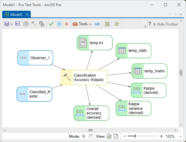
For ModelBuilder chains the tool offers six outputs: the optional report file, per-class statistics table and error-matrix table, plus three derived scalars — Kappa, its variance, and overall accuracy — so a model can branch on accuracy thresholds, collect results across candidate models, or feed the Compare Accuracy Analyses tool directly (with an analysis field, the derived values carry the first analysis):
Parameters
| Label | Explanation | Data type |
|---|---|---|
| Sample points or tableRequired · in_features | The reference samples: a point layer (required when classes are extracted from layers) or any table whose rows pair predicted and observed classes. A selection is honored. | Feature Layer; Table View |
| Classification (predicted) data source attribute fieldOptional · predicted_field | The attribute field from the sample points attribute table holding each sample's predicted class. Give either this field or the classified dataset below. | Field |
| Classification (predicted) raster or polygon feature classOptional · predicted_layer | The classified dataset itself: an integer raster (cell values = classes — continuous floating-point rasters are refused; classify them first) or polygons with a class field. Values are extracted at each sample point. This dataset also supplies the class proportions for the area-weighted estimates: the tool measures each class's share of the dataset's ground area — geodesic polygon areas summed per class, or cell counts per class (latitude-corrected on geographic rasters), over the analyzed classes only — and those shares become the strata weights of the Card/Olofsson block. | Raster Layer; Feature Layer |
| Class field of the classification (predicted) datasetOptional · predicted_class_field | For a polygon feature class: the attribute field holding the class value (required). For a raster: optionally a raster attribute-table field — typically the class-name field — so the extracted classes match a reference field that stores names rather than the cell codes. Blank uses the raw cell values. | Field |
| Observed (reference) data source attribute fieldOptional · observed_field | The attribute field from the sample points attribute table holding each sample's observed (field-verified, reference) class. Give either this field or the dataset below. | Field |
| Observed (reference) classified raster or polygon feature classOptional · observed_layer | The classified raster (integer cell values; continuous floating-point rasters are refused) or polygon feature class holding the reference classes, extracted at each sample point. | Raster Layer; Feature Layer |
| Class field of the observed (reference) datasetOptional · observed_class_field | For a polygon feature class: the attribute field holding the class value (required). For a raster: optionally a raster attribute-table field (e.g. a class-name field) so the extracted classes match the predicted side's vocabulary. Blank uses the raw cell values. | Field |
| Output report fileOptional output · out_report | A text file holding the complete report — the error
matrix, every statistic with its interval, the comparisons, and the
ready-to-run R snippet. The .txt extension is added
automatically if omitted. The full report also prints in the
messages. |
File |
| Output per-class statistics tableOptional output · out_class_table | One row per class (per analysis): sample counts, user's/producer's accuracies, conditional kappa with SE, sensitivity, specificity, predictive powers, F1, and — when weighted — the area-weighted accuracies with SEs and the error-adjusted area estimates. Join it back to your classified layer to symbolize accuracy. A table written to a folder is a dBASE (.dbf) table, which cannot store nulls: a statistic that is undefined there is written as −999. In a geodatabase table it is null. | Table |
| Output error-matrix tableOptional output · out_matrix_table | The error matrix as a long table (Analysis, Predicted, Observed, Count) for further analysis or charting. | Table |
| Analysis fieldOptional · analysis_field | Split the samples into separate analyses — per observer, per model, per year. Each gets its own full report block, and all are compared: pairwise Z tests plus the Fleiss common-kappa chi-square test. | Field |
| Circle radius for locational uncertaintyOptional · circle_radius | Extract the majority class in a circle of this radius around each sample instead of the value exactly at the point — the conservative choice when sample coordinates carry GPS error. Ties go to the value at the point. Applies to layer-extracted values only. | Double |
| Units for the circle radiusOptional · linear_units | Meters, Kilometers, Feet or Miles. | String |
| Ordinal weighting for weighted kappaOptional · weighting | For ordinal classes (suitability ranks, cover classes): add Cohen's weighted kappa, where near-misses count more than gross errors. Linear weights disagreements by rank distance; quadratic by its square (more forgiving of adjacent-rank confusion). Classes are ranked in their sorted order. | String |
| Confidence level (percent, 0 - 100)Optional · confidence | The confidence level for every interval in the report (default 95). | Double |
| Weight the analysis by map class proportionsOptional · weight_by_map | Adds the area-weighted block: Card (1982) / Olofsson et al. (2014) stratified accuracies with standard errors and the error-adjusted area estimates with confidence intervals — the estimates current journals expect. Proportions come from the classification (predicted) dataset automatically, or from the override table below. | Boolean |
| Sampling design of the reference samplesOptional · design | How the reference samples were drawn — stratified random by map class (each class sampled separately; the usual accuracy-assessment design) or simple random over the whole classified area. The variance formulas differ (Card 1982). | String |
| Map class proportionsOptional · map_props | Optional override: type each class's proportion (or area — values are normalized). When blank, proportions are computed from the classification (predicted) dataset: geodesic areas for polygons, latitude-corrected cell counts for rasters. With neither, the sample's own predicted-class proportions are used with a warning. | Value Table |
| Total map area in hectaresOptional · map_area_ha | Normally left blank: the tool measures the total mapped area automatically from the classification (predicted) dataset — the area of the analyzed classes, NoData excluded; geodesic for polygons, cell size times count for projected rasters, latitude-corrected cell areas for geographic rasters (estimated from the cell area at the raster's central latitude when the classes are read through an attribute-table field). Enter a value here only if you want to override the auto-calculated map area. For example, if you have an official map area, or if you are using data that can't tell you the area (such as if both your classification and sampled points are from a point feature class attribute table, and you therefore have no raster or polygon feature class that clearly shows the area; map proportions typed by hand likewise carry no area). | Double |
| Bootstrap replicatesOptional · boot_reps | The number of bootstrap resamples used to build percentile confidence intervals for kappa and overall accuracy; leave blank to skip. Each replicate redraws the full number of samples with replacement from the original samples and recomputes the statistics. 1,000 to 2,000 replicates is the usual choice. Most useful when the normal approximation is doubtful (see Usage). | Long |
| Random seed (bootstrap)Optional · random_seed | The same seed reproduces the same bootstrap intervals exactly. | Long |
Derived outputs (ModelBuilder)
| Label | Explanation | Data type |
|---|---|---|
| Kappa (derived)out_kappa | Cohen's Kappa of the analysis (the first analysis when an analysis field produces several). | Double |
| Kappa variance (derived)out_kappa_var | The Fleiss-Cohen-Everitt delta-method variance of kappa — paired with kappa, it feeds the Compare Accuracy Analyses tool. | Double |
| Overall accuracy (derived)out_overall | The overall proportion of correctly classified samples. | Double |
Python
Import the toolbox once, then call the tool like any geoprocessing tool (parameter names as in the tables above):
import arcpy
arcpy.ImportToolbox(r"C:\path\to\JennessEnterprisesTools.pyt")  # your install path
arcpy.jenness.ClassificationAccuracy(
    in_features=r"D:\data\accuracy.gdb\field_plots",
    predicted_layer=r"D:\data\accuracy.gdb\veg_classification",
    observed_field="Field_Class",
    circle_radius=15.0, linear_units="Meters",
    weight_by_map=True,
    out_report=r"D:\data\accuracy_report.txt",
    out_class_table=r"D:\data\accuracy.gdb\class_stats",
    out_matrix_table=r"D:\data\accuracy.gdb\error_matrix")
Recommended citation
Credits and references
By Jeff Jenness, Jenness Enterprises
(www.jennessent.com), and
J. J. Wynne, Department of Biological Sciences and Center for
Adaptive Western Landscapes, Northern Arizona University. A modernized
port of: Jenness, J. and J. J. Wynne (2007), Cohen's Kappa
and classification table metrics 2.1a (kappa_stats.avx), Jenness
Enterprises. Algorithms validated against the R packages
psych, caret, yardstick,
mapaccuracy, diffeR and irrCAC.
- Card, D. H. 1982. Using known map category marginal frequencies to improve estimates of thematic map accuracy. Photogrammetric Engineering and Remote Sensing 48:431–439. ntrs.nasa.gov/citations/19820041921
- Congalton, R. G., and K. Green. 1999. Assessing the Accuracy of Remotely Sensed Data: Principles and Practices. Lewis Publishers.
- Foody, G. M. 2020. Explaining the unsuitability of the kappa coefficient in the assessment and comparison of the accuracy of thematic maps obtained by image classification. Remote Sensing of Environment 239:111630. doi.org/10.1016/j.rse.2019.111630
- Gwet, K. L. 2008. Computing inter-rater reliability and its variance in the presence of high agreement. British Journal of Mathematical and Statistical Psychology 61:29–48. doi.org/10.1348/000711006X126600
- Olofsson, P., G. M. Foody, M. Herold, S. V. Stehman, C. E. Woodcock, and M. A. Wulder. 2014. Good practices for estimating area and assessing accuracy of land change. Remote Sensing of Environment 148:42–57. doi.org/10.1016/j.rse.2014.02.015
- Pontius, R. G., Jr., and M. Millones. 2011. Death to Kappa: birth of quantity disagreement and allocation disagreement for accuracy assessment. International Journal of Remote Sensing 32:4407–4429. doi.org/10.1080/01431161.2011.552923
- Stehman, S. V., and G. M. Foody. 2019. Key issues in rigorous accuracy assessment of land cover products. Remote Sensing of Environment 231:111199. doi.org/10.1016/j.rse.2019.05.018
Licensing information
Works at every ArcGIS Pro license level (Basic, Standard, Advanced). No extension licenses are required — by contrast, Esri's Compute Confusion Matrix requires Spatial Analyst or Image Analyst.
Related tools and pages
- About Kappa and classification accuracy analysis — the theory behind every statistic this tool reports.
- Kappa analysis tutorial — a complete worked assessment on the Pinaleños dataset.
- Footnotes — what the cited authors actually said, verbatim.
- Estimate Sample Size — how many reference samples the assessment needs, by four methods.
- Random Point Generator and Select Random Records — draw the reference design.
- Compare Accuracy Analyses — compare kappas from separate runs or from the literature.
- Cross-Tab Statistics — a plain contingency table without inference.