

General Raster Classification
Summary
Classifies any single-band raster into named, colored categories using a saved general classification system: a set of threshold rules on the raster's own values, or on its whole-raster standardized (z-score) values. It is the general-purpose sibling of the Slope Position Classification and Landform Classification tools: the same reusable classification systems and the same per-user store, applied to an arbitrary raster rather than to a DEM. Elevation, a slope raster, a wetness index, a habitat-suitability surface, a model output: anything with one band can be classified. The output is an integer raster with a Value and Class_Name attribute table and the system's color map, so it draws as named classes the moment it is added to the map. No Spatial Analyst or 3D Analyst extension is required.
If you know Esri's Reclassify tool
This tool serves a similar purpose to Esri's standard Reclassify tool: it turns a continuous raster into integer classes, so much of what you expect from Reclassify applies here. The differences are these:
- The classification scheme is not typed into the tool dialog each time. It is created once, as a reusable named system, in the standalone Classification System Builder, and then simply picked from a dropdown here.
- Each output class stores a name, and a display color, with the raster's attribute table, so the result draws and reads as named, colored categories rather than bare integers.
- No additional extension is required. Esri's Reclassify needs a Spatial Analyst or 3D Analyst license; this tool runs on any ArcGIS Pro license.
- Classes can be defined in standardized units as well as in the raster's own values: thresholds in standard deviations from the mean of the whole raster, so that “more than one standard deviation above average” can be a class without first working out what value that is. Reclassify works only in the raster's own values.
The tool is the direct descendant of the General Grid Classification function in the Topographic Position Index extension for ArcView 3.x (Jenness 2006). It is renamed here because grid was the raster format of the ArcView and ArcInfo era, and the word means little to newer users.
How a class is defined
A general classification system holds one or more classes, each with a value, a name, a color, and one criterion on the input raster. The criterion is a threshold condition, such as value > 1, or a range made of two conditions joined by and or or, such as value > −1 and value ≤ 0. A cell takes a class when its criterion holds: the single condition, or the two conditions combined by the and or or chosen. Where two classes overlap, the class with the lower value wins, so class values also set precedence. A cell that matches no class, or that is NoData in the input, is written as unclassified: value 0, which the output treats as NoData.
The thresholds may be read in either of two ways, and the system records which. Raw thresholds are compared with the raster's own values, in its own units, so they are absolute: a threshold of 30 on a percent-slope raster means 30 percent wherever it occurs. Standardized thresholds are compared with the whole-raster z-score of each cell,
where the mean and standard deviation are those of every valid cell in the input raster. A standardized threshold of 1 therefore means one standard deviation above the raster's mean, whatever the raster's units and range. Standardized thresholds adapt to the raster's own distribution, which is useful when the value range is not known in advance, or when the same system is to be applied to rasters with different ranges; raw thresholds are the choice when the numbers themselves carry meaning. Classification is a single vectorized pass in numpy over the whole raster, with no Esri Con and no Spatial Analyst.
The three bundled templates
Three general systems ship with the add-in. Two use standardized bands and are meant as generic starting points; the third, a forestry slope classification in raw percent, is described in the worked example below. Open any of them in the Classification System Builder, duplicate it, and edit the thresholds, units, names and colors for your own data.
| Value | Class name | Criterion (standardized) | Color |
|---|---|---|---|
| 1 | Low | z ≤ −1 | 44, 123, 182 |
| 2 | Below Average | −1 < z ≤ 0 | 171, 217, 233 |
| 3 | Above Average | 0 < z ≤ 1 | 253, 174, 97 |
| 4 | High | z > 1 | 215, 25, 28 |
| Value | Class name | Criterion (standardized) | Color |
|---|---|---|---|
| 1 | Very Low | z ≤ −1.5 | 69, 117, 180 |
| 2 | Low | −1.5 < z ≤ −0.75 | 145, 191, 219 |
| 3 | Below Average | −0.75 < z ≤ −0.25 | 224, 243, 248 |
| 4 | Average | −0.25 < z ≤ 0.25 | 255, 255, 191 |
| 5 | Above Average | 0.25 < z ≤ 0.75 | 254, 224, 144 |
| 6 | High | 0.75 < z ≤ 1.5 | 252, 141, 89 |
| 7 | Very High | z > 1.5 | 215, 48, 39 |
Every general system you create or edit in the Builder appears in this tool's dropdown alongside these three. Systems are stored as JSON files in a per-user folder that survives add-in reinstalls, and a system can be shared with a colleague by copying its file.
A worked example: slope classes for forest operations
The two standardized templates suit any raster whose range you do not know in advance. Raw thresholds are the other half of the tool, and a slope raster is the clearest case for them. A forester does not want “one standard deviation above the average slope on this particular DEM,” a value that moves every time the analysis extent changes; a forester wants the slope at which a rubber-tired skidder stops being an option. Those numbers are fixed, they are published, and they mean the same thing on every map.
The third bundled system, Ground-Based Equipment Operability (Percent Slope), classifies a percent-slope raster into six bands of ground-based equipment operability. Each break is a value that appears in published Forest Service or state direction, cited at the end of this section. Because the thresholds are raw, the system applies unchanged to every project area.
| Value | Class name | Criterion (raw, percent) | What it means on the ground | Color |
|---|---|---|---|---|
| 1 | Unrestricted Ground-Based | value ≤ 20 | Conventional ground-based equipment is permitted on slopes of less than 20 percent even where soil survey data are unavailable (GMUG forest plan). | 69, 117, 180 |
| 2 | Ground-Based, Wheeled Limit | 20 < value ≤ 30 | The Oregon OSHA limit for rubber-tired skidders, and the general limit for ground-based mechanized vegetation treatment in the Lake Tahoe Basin Management Unit plan. | 145, 191, 219 |
| 3 | Tracked Equipment Only | 30 < value ≤ 40 | The Oregon OSHA limit for crawler tractors, tracked feller bunchers, tracked excavators and loaders; also the GMUG plan's limit for conventional equipment where soil data are available. | 224, 243, 248 |
| 4 | Steep-Slope Equipment | 40 < value ≤ 50 | The Oregon OSHA limit for forestry equipment designed for steep slopes. In the SBEADMR analysis, mechanical treatment above 40 percent was limited to chainsaws. | 254, 224, 144 |
| 5 | Tethered or High-Flotation | 50 < value ≤ 60 | High-flotation equipment to 60 percent (GMUG plan); cut-to-length systems travelling on a slash mat to 60 percent (SBEADMR). | 252, 141, 89 |
| 6 | Cable, Aerial or Hand Only | value > 60 | Beyond the documented ground-based limits. Cable and aerial systems may be used on any slope (GMUG plan); otherwise hand treatment or prescribed fire. | 215, 48, 39 |
These thresholds are in percent slope, the unit forest operations direction is written in. A slope raster in degrees needs a second classification system built with the equivalent breaks: 20 percent = 11.3°, 30 = 16.7°, 40 = 21.8°, 50 = 26.6°, 60 = 31.0°. Raw thresholds are compared with the raster's own values, so the tool cannot detect a unit mismatch: a degree raster run against this system puts far too much ground in the gentle classes, because every slope is a smaller number in degrees than in percent. Naming the slope raster for its units is the simplest guard against it.
Obviously, getting the units right matters in general, not just for slope: classifying a DEM in feet against elevation thresholds written in meters causes exactly the same kind of problem.
Because every class carries its own color and opacity, the output drawn over a hillshade is a finished operability map with no symbolization step. Setting class 1 to partial opacity in the Classification System Builder lets the gentle ground read as terrain while the constrained classes stay solid.
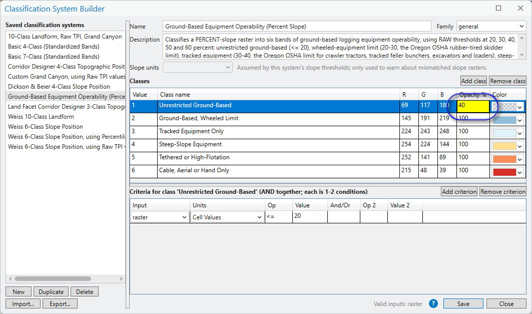
The same Color Editor is available after the output is on the map. The classified raster is an ordinary layer, so any class's color and transparency can be changed from the layer's Symbology pane in the same way, without touching the classification system: useful for adjusting one map without changing the defaults every future run will use.
import arcpy
arcpy.ImportToolbox(r"C:\path\to\JennessEnterprisesTools.pyt")  # your install path

# The input must be a PERCENT-slope raster; see the note on units above.
arcpy.jenness.GeneralRasterClassification(
    in_raster=r"D:\Project.gdb\Percent_Slope",
    out_raster=r"D:\Project.gdb\Slope_Operability_Classes",
system="Ground-Based Equipment Operability (Percent Slope)")Sources for the thresholds
- Oregon OSHA. 2016. Oregon OSHA's revised guidelines for using tethered logging systems. Quotes OAR 437-007-0935(1): machines must not be operated on slopes in excess of 30 percent for rubber-tired skidders; 40 percent for crawler tractors, tracked feller bunchers, tracked excavators and loaders; and 50 percent for other forestry equipment designed for steep slopes, unless specified by the equipment's manufacturer. osha.oregon.gov (PDF)
- Tahoe Regional Planning Agency. 2020. Initial Determination of Environmental Impact Checklist. Proposed Code Amendments: Allowing Ground-based Mechanical Equipment on Slopes between 30 and 50 percent. Quotes the Lake Tahoe Basin Management Unit 2016 Land Management Plan (“In general, operate ground-based mechanized equipment for vegetation treatment on slopes less than or equal to 30%”) and the California Forest Practice Rules (except for tethered operations, heavy equipment prohibited on slopes steeper than 65 percent, or steeper than 50 percent where the erosion hazard rating is high or extreme). trpa.gov (PDF)
- USDA Forest Service. Forest Operations Equipment Catalog: Tethered Logging Systems. Reports the Oregon OSHA equipment slope limits above, and advises operators to adhere to the maximum slope specified by the equipment's manufacturer. fs.usda.gov/forestmanagement/equipment-catalog/tethered.shtml
- USDA Forest Service, Grand Mesa, Uncompahgre and Gunnison National Forests. 2022. SBEADMR Supplemental Information Report on Cut-to-Length and Tethered Logging Technologies. Quotes the forest plan (III-41 to III-42): conventional logging equipment on slopes of less than 20 percent where soil data are unavailable, up to 40 percent where they are available, high-flotation equipment to 60 percent, and cable and aerial systems on any slope; the SBEADMR analysis limiting mechanical treatment above 40 percent to chainsaws; and cut-to-length systems travelling on a slash mat accepted to 60 percent. cfri.colostate.edu (PDF)
- USDA Forest Service, Kaibab National Forest. Steep Slope Forest Restoration. Notes that hazardous fuels reduction on steep slopes “requires technical operations with specialty equipment that is not commonly used nor readily accessible in the Southwest.” fs.usda.gov/r03/kaibab
A tour of the dialog
The example classifies percent slope on the Coconino National Forest around the San Francisco Peaks, north of Flagstaff, with the Ground-Based Equipment Operability (Percent Slope) system described above, its first class set to partial opacity.
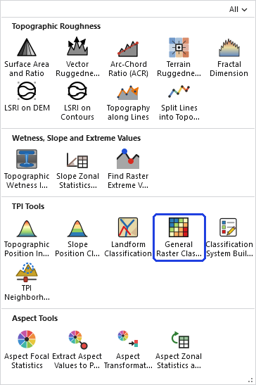
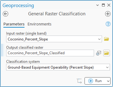
The dialog asks for three things: the raster to classify, a name for the output, and the classification system to apply. The system list is read from the per-user store each time the dialog opens, so a system saved in the Builder a moment ago is already there. The output name is suggested from the input.
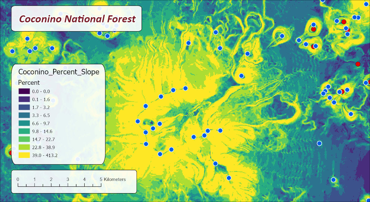
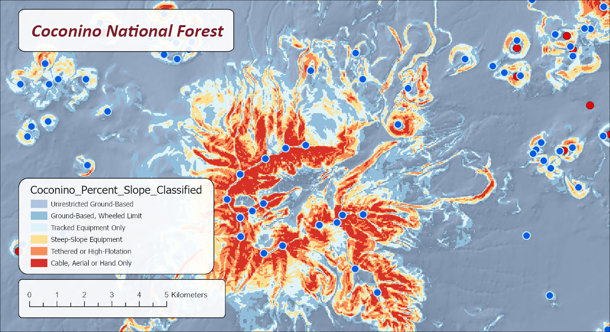
The output carries its classes with it. Its attribute table has a Value and a Class_Name field, one row per class that occurs, and its color map holds the system's colors, including any per-class opacity set in the Builder, so a hillshade beneath can show through selected classes. Added to a map, it draws as named, colored categories with no symbolization step.
The tool holds the whole raster in memory at once, so the memory it needs grows with the number of cells. On most rasters that is no concern. On a very large one the tool may need more memory than your computer has free, and then one of two things happens: Windows starts using the disk as overflow memory and the tool slows to a crawl, or the tool stops with an out-of-memory error. There is no fixed limit; it depends on how much memory your computer has free. If a raster is too large, clip it to the area you need first.
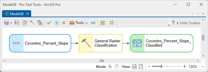
ModelBuilder
Parameters
| Label | Explanation | Data type |
|---|---|---|
| Input raster (single band)Required · in_raster | Any single-band raster to classify. Its values are read as they are for raw thresholds, or standardized over the whole raster for standardized thresholds, as the chosen classification system specifies. | Raster Layer; Raster Dataset |
| Output classified rasterRequired · out_raster | The output integer class raster, carrying a Value and Class_Name attribute table and a color map from the classification system, including any per-class opacity. Cells matching no class, or outside the data, are unclassified. A name is suggested from the input. | Raster Dataset |
| Classification systemRequired · system | The saved general classification system to apply: its thresholds, names and colors. This plays the role of the remap table you would type into Esri's Reclassify tool, except that it is created once in the Classification System Builder and reused, and it carries a name and color for each class. The list is read from the per-user store; the bundled defaults are the Basic 4-Class and Basic 7-Class standardized-band templates and the Ground-Based Equipment Operability (Percent Slope) system. | String |
Python
The system is named exactly as it appears in the Builder. Any
general system you have created is valid; the comment block lists
only the bundled ones. The names of the
systems on your computer are listed in the
Classification System
Builder; they are also the "name" entries of the
JSON files in
%LOCALAPPDATA%\JennessEnterprises\WildlifeTools\classification_systems\,
but if you look them up there, take care not to change anything: an
edited file can leave a system unreadable.
import arcpy
arcpy.ImportToolbox(r"C:\path\to\JennessEnterprisesTools.pyt")  # your install path

# ---- valid options for the list-driven parameter -------------------------
# system (bundled; user-created systems from the Classification System
#         Builder are also valid -- this list is not exhaustive):
#                      "Basic 4-Class (Standardized Bands)"
#                      "Basic 7-Class (Standardized Bands)"
#                      "Ground-Based Equipment Operability (Percent Slope)"

arcpy.jenness.GeneralRasterClassification(
    in_raster=r"D:\Flagstaff.gdb\Flagstaff_Percent_Slope",
    out_raster=r"D:\Flagstaff.gdb\Slope_7_Classes",
    system="Basic 7-Class (Standardized Bands)")
Recommended citation
Credits and references
By Jeff Jenness, Jenness Enterprises (www.jennessent.com), modernizing the General Grid Classification function of his Topographic Position Index extension for ArcView 3.x, which automated the classification methods of Weiss (2001).
- Jenness, J. 2006. Topographic Position Index (tpi_jen.avx) extension for ArcView 3.x, v. 1.3a. Jenness Enterprises. jennessent.com/arcview/tpi.htm
- Oregon OSHA. 2016. Oregon OSHA's revised guidelines for using tethered logging systems. Oregon Occupational Safety and Health. osha.oregon.gov (PDF)
- Tahoe Regional Planning Agency. 2020. Initial Determination of Environmental Impact Checklist. Proposed Code Amendments: Allowing Ground-based Mechanical Equipment on Slopes between 30 and 50 percent. Tahoe Regional Planning Agency. trpa.gov (PDF)
- USDA Forest Service. Forest Operations Equipment Catalog: Tethered Logging Systems. USDA Forest Service. fs.usda.gov/forestmanagement/equipment-catalog/tethered.shtml. Accessed on 27 September 2026.
- USDA Forest Service, Grand Mesa, Uncompahgre and Gunnison National Forests. 2022. SBEADMR Supplemental Information Report on Cut-to-Length and Tethered Logging Technologies. USDA Forest Service. cfri.colostate.edu (PDF)
- USDA Forest Service, Kaibab National Forest. Steep Slope Forest Restoration. USDA Forest Service. fs.usda.gov/r03/kaibab. Accessed on 27 September 2026.
- Weiss, A. 2001. Topographic Position and Landforms Analysis. Poster presentation, ESRI User Conference, San Diego, CA. jennessent.com/arcview/TPI_Weiss_poster.htm
Licensing information
Works at every ArcGIS Pro license level (Basic, Standard, Advanced). No extension licenses are required; the classification is computed internally, without Spatial Analyst or 3D Analyst.
Related tools and pages
- About TPI — the Topographic Position Index family of tools and how they fit together.
- Classification System Builder — author and edit the systems this tool applies.
- Topographic Position Index — compute TPI rasters, which this tool can classify with a general system.
- Slope Position Classification — the same machinery applied to TPI plus slope.
- Landform Classification — the same machinery applied to TPI at two scales plus slope.
- TPI Neighborhood Sampler — try neighborhood sizes and thresholds on a snapshot of the DEM, with sliders, before running the tools.