

Aspect Zonal Statistics as Table
Summary
Summarizes an aspect raster within zones and writes the results to a table of circular statistics: one row per zone, holding the mean direction, the resultant length and mean resultant length, the circular variance and standard deviation, the angular variance and deviation, the median direction, the circular range, the von Mises concentration, the Rayleigh test of uniformity, and the 95% confidence interval of the mean direction. The zones can be an integer raster or a point, polyline or polygon feature class. The tool is modeled on Esri's Zonal Statistics as Table, but aspect is a direction, and directions wrap around: 359° and 1° are two degrees apart, not 358. Ordinary statistics get that wrong, so every statistic here is a circular one. Flat cells, which face no direction at all, are left out of the statistics and counted separately. No Spatial Analyst or Image Analyst extension is needed; every calculation is done internally.
Why aspect needs circular statistics
Aspect is the compass direction the ground faces, measured clockwise from north: 0° is north, 90° east, 180° south, 270° west, and 360° is north again. The number line of ordinary statistics has two ends; the compass does not (Jenness 2012). Take the simplest possible zone, two cells facing just either side of north:
| Two cells | Arithmetic mean | Circular mean |
|---|---|---|
| 350° and 10° | 180° (due south) | 0° (due north) |
| 359° and 1° | 180° (due south) | 0° (due north) |
Both cells face very nearly north, and the arithmetic mean says the zone faces due south, the one direction neither cell comes close to. That is not a rounding problem; it is what averaging does to numbers that wrap around. The ordinary standard deviation fails the same way: the two cells in the first row are 20° apart on the ground and 340 apart on the number line. With its default settings, Esri's Zonal Statistics as Table computes MEAN and STD on the raw cell values, so on an aspect raster any zone that faces anywhere near north gets a meaningless mean. (Its Calculate circular statistics option avoids this; see Compared with Esri's tool.)
The vector mean
The circular statistics start from a different idea. Treat each cell's aspect θ as an arrow of length one pointing in that direction, with an east-west component sin θ and a north-south component cos θ. Add up all the arrows. The direction of the sum is the mean direction, and the length of the sum says how much the arrows agreed. For the n directional cells of a zone:
Here S̄ and C̄ are the mean sine and mean cosine, R̄ is the mean resultant length (r-bar), the length of the average arrow, and θ̄ is the mean direction, the compass direction of that average arrow; atan2 is the two-argument arctangent that returns the full 0° to 360° circle. The resultant length itself, R, is the length of the summed arrow, n times R̄.
The mean resultant length runs from 0 to 1 and is the single most useful number in the table. At 1, every cell in the zone faces exactly the same way. Near 0, the arrows cancel: the cells face every direction about equally, as on a rounded summit, or face two opposite ways equally, as in a symmetric valley whose two walls face east and west. When R̄ is near 0 the mean direction is close to meaningless, since it is the direction of an arrow with almost no length; when the summed arrow has no length at all, the tool leaves the mean direction NULL.
A worked example
Five cells of a zone that faces roughly north, three of them just east of north and two just west of it:
| Aspect θ | sin θ (east-west) | cos θ (north-south) |
|---|---|---|
| 340° | −0.3420 | 0.9397 |
| 355° | −0.0872 | 0.9962 |
| 5° | 0.0872 | 0.9962 |
| 20° | 0.3420 | 0.9397 |
| 30° | 0.5000 | 0.8660 |
| Mean | S̄ = 0.1000 | C̄ = 0.9476 |
The mean arrow points a little east of north: its direction is atan2(0.1000, 0.9476) = 6.0°, and its length is R̄ = 0.953, close to 1, because the five cells agree closely. The arithmetic mean of the five numbers is 150°, south-southeast. The tool's other statistics for these five cells, computed by the tool's own code, are in the next table.
The statistics
The statistics follow Mardia and Jupp (2000), Fisher (1993) and Batschelet (1981). The table gives each statistic briefly, with its value for the five-cell example above; About Aspect discusses them more thoroughly, including the vector mean, the measures of dispersion and concentration, the Rayleigh test and the confidence interval, and how to read the mean resultant length.
| Statistic (field) | How it is computed | Worked example |
|---|---|---|
| Mean Direction (MEAN_DIR) | The direction of the summed unit vectors, 0° to 360°, as above. | 6.02° |
| Mean Resultant Length (RBAR) | The length of the mean unit vector, 0 to 1. | 0.9528 |
| Resultant Length (R_LENGTH) | The length of the summed vector, n × R̄. | 4.764 |
| Circular Variance (CIRC_VAR) | 1 − R̄, from 0 (identical) to 1 (no concentration). | 0.0472 |
| Angular Variance (ANG_VAR) | 2(1 − R̄), in squared radians. | 0.0944 |
| Circular Standard Deviation (CIRC_SD) | √(−2 ln R̄), converted to degrees. | 17.81° |
| Angular Deviation (ANG_DEV) | √(2(1 − R̄)), converted to degrees. | 17.60° |
| Median Direction (MEDIAN_DIR) | The observed direction with the least total circular distance to all the others, found on a 0.1° histogram and reported as the center of its 0.1° bin. | 5.05° |
| Circular Range (CIRC_RANGE) | The smallest arc that contains every observation: 360° minus the largest empty gap, at 0.1° resolution. | 50.0° |
| von Mises Concentration (VM_KAPPA) | κ, the concentration parameter of the von Mises distribution, the circular counterpart of the normal distribution, estimated from R̄ by the piecewise approximation of Best and Fisher (1981, p. 495), also given by Fisher (1993, equation 4.40), with the small-sample correction Best and Fisher propose (p. 498; Fisher 1993, equation 4.41) for zones of 15 or fewer directional cells; capped at 10,000. | 5.35 (10.87 before the correction) |
| Rayleigh Test (RAYLEIGH_Z, RAYLEIGH_P) | Z = nR̄², and the probability of a resultant that long if the directions were uniformly spread around the circle, from Zar (1999) equation 27.4. | Z = 4.54, p = 0.0041 |
| 95% Confidence Interval (CI95_HALF, CI95_LO, CI95_HI) | Half-angle arcsin(1.96 / √(n R̄ κ)), from the von Mises standard error (Fisher 1993, equations 4.42 and 4.43), in degrees, with the lower and upper bounds of the mean direction. | ±22.85°, 343.18° to 28.87° |
The dispersion measures come in two families, and the difference matters mostly when the directions are widely spread. The circular variance and the angular variance and deviation are simple functions of R̄; the circular standard deviation uses its logarithm, grows without limit as R̄ approaches 0, and is the closer analog of an ordinary standard deviation for concentrated data. In the worked example, with the cells tightly grouped, the circular standard deviation and the angular deviation are nearly the same, 17.8° and 17.6°. The median and range are order statistics, computed on a 0.1° histogram of each zone's directions, which is why the example's median reads 5.05°, the center of the bin holding the observed 5°.
The Rayleigh test asks whether a zone has any preferred direction at all. Its null hypothesis is that the aspects are spread uniformly around the circle; a small p says the zone faces somewhere in particular. The p value is Zar's (1999) equation 27.4, which he gives as derived from Greenwood and Durand (1955). Greenwood and Durand give the exact distribution by numerical integration, with tables, and a series expansion in powers of 1/n (their eq. 6.4, p. 242); the closed form itself does not appear in their paper. With R = nR̄ is
the same formula the Topography along Lines tool uses for its Rayleigh test. The five cells of the example give p = 0.0041. The half-angle is an arcsine, and an arcsine exists only for values up to 1, so the interval exists only while the standard error of the mean direction is less than 1 / 1.96, about 0.51 radians or 29°. Beyond that the directions are too dispersed for an interval, and the three fields are left empty. Fisher (1993, Table 4.3) recommends this interval only when the concentration is strong enough for the sample size: for any sample when κ is 2 or more, for at least 10 directions when κ is between 1.5 and 2, at least 15 when it is between 1 and 1.5, and at least 25 when it is between 0.4 and 1. Below 0.4 he advises a bootstrap interval instead, whatever the sample size. The tool computes the interval outside that range too, and its messages say how many zones are affected. They also say how many zones had 15 or fewer directional cells and so carry the small-sample correction of κ.
Both the Rayleigh test and the confidence interval assume that every aspect value is an independent observation, and for zones from an integer raster or from polygons or polylines that assumption fails badly. Neighboring cells face nearly the same way, partly because hillsides are continuous and partly because each cell's aspect is computed from a 3 × 3 window of elevations that its neighbors share. On the Coconino slope raster used on the Slope Zonal Statistics as Table page, even the slopes of cells 2.8 km apart are still correlated. A zone of thousands of correlated cells carries far less independent information than its cell count suggests, so almost any zone that faces anywhere tests significant, and the interval is much narrower than the real uncertainty of the mean direction; read it as a lower bound, useful mainly for comparing zones of similar size. And when the cells are all the cells in the zone, the tool has taken a census: the zone's mean direction is simply known, and neither the test nor the interval has anything to estimate unless the cells are treated as a sample of some larger process. R̄ and the standard deviations, which describe how variable the directions are, are not affected by any of this.
Point zones are a different case. Each point contributes a single interpolated direction, and points spread farther apart than the distance over which aspects stay correlated, such as survey plots or randomly placed sample locations, can well be independent observations; for those, the Rayleigh test and the interval mean what they say. Points crowded close together share the cells' autocorrelation, and the same caution applies.
Flat cells
Esri's Aspect tool gives a flat cell the value −1. A flat cell faces no direction, so it cannot take part in directional statistics, and counting −1 as a direction would corrupt every one of them. The tool therefore leaves flat cells out of the statistics, and says so when it runs, but it never discards them silently: every zone's flat cells are counted in FLAT_COUNT and reported in FLAT_PCT as a percentage of the zone's directional and flat cells together. A zone that is mostly flat therefore announces itself, and a mean direction computed from a handful of cells in a mostly flat zone can be read with the caution it deserves. Values outside the range −1 to 360, which an aspect raster should never contain, are excluded as well, counted, and reported with a warning that the raster might not be an aspect raster. Esri's circular option does none of this: it treats −1 as an angle, which wraps to 359°, so every flat cell counts as facing a degree west of north (see below).
Direction conventions and flow direction rasters
The Input aspect convention drop-down says how the raster measures direction. Compass (0 = north, clockwise), the default, is ordinary aspect. Mathematical (0 = east, counter-clockwise; e.g. D-infinity) is the convention of D-infinity flow-direction rasters, whose values are the direction of steepest descent and so are essentially aspect measured the other way. With the mathematical convention, each value is converted to a compass direction before any statistic is computed. The convention affects only the direction-valued outputs: the mean and median direction and the confidence bounds. The resultant length, the variances and deviations, the range, kappa and the Rayleigh test are identical under either.
The tool sets the drop-down for you when it can, by reading the geoprocessing history stored in the raster's metadata: a raster produced by Esri's Flow Direction tool with the D-infinity option is recognized, and the drop-down falls back to Compass when the history says nothing. A raster from Flow Direction's D8 option is a different matter. Its values, 1, 2, 4, 8, 16, 32, 64 and 128, are codes for eight categories, not angles, and statistics on them are meaningless; the tool warns when the raster's geoprocessing history says it came from Flow Direction's D8 option.
Zones
Zones can come from an integer raster, where every distinct cell value is a zone, or from a point, polyline or polygon feature class or layer, where all features sharing the same value in the Zone field form one zone. A zone raster must be an integer raster in the same coordinate system as the aspect raster. Integer, text, GUID and ObjectID fields all work as zone fields; choosing the ObjectID makes every feature its own zone. An active selection on a layer is honored.
A feature layer with a table joined to it works too: the joined fields appear in the zone-field list under their qualified names, such as lookup.Unit, and any of them can define the zones. A raster zone always uses its cell values, so the zone field for a zone raster is always Value.
Feature zones are processed one zone at a time, each over its own window of the aspect raster, so zones that overlap are each analyzed in full, and within one zone, features that overlap each other count each cell once. Earlier versions of Esri's zonal tools rasterized the zones first, so that one of two overlapping polygons silently lost the cells they shared; the current Esri tool analyzes overlapping features individually too, and gave the same counts as this tool in a test in ArcGIS Pro 3.7.
How a feature claims cells depends on its geometry:
- Polygons use every cell whose center falls inside the polygon.
- Polylines use every cell the line passes through.
- Points take the aspect at the point itself, as a bilinear weighted mean direction of the four surrounding cell centers: each neighbor's unit vector is weighted by the ordinary bilinear weights and the resultant turned back into a direction, so a point among cells at 358°, 359°, 1° and 2° interpolates to about 0°, never 180°. Flat and NoData neighbors are left out with the weights renormalized, and a point whose neighbors are all flat counts as flat.
Zones that lie entirely outside the raster do not appear in the output table, matching the Esri tool's behavior of working on the intersection of the extents. Polygons stored with true curves, such as the circles a geodatabase Buffer produces, are densified automatically before their cells are gathered. If Ignore NoData in calculations is unchecked, any zone containing even one NoData cell receives NULL statistics, again matching the Esri tool with the same setting; checked, the default, NoData cells are simply skipped.
The output table
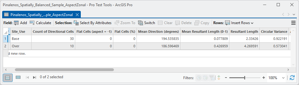
The table has one row per zone. Its fields, in order, are the zone value (named after the zone field), COUNT (the number of directional cells used), FLAT_COUNT, FLAT_PCT, and then whichever statistics were requested, with the field names shown in the statistics table above. The three count fields are always written. A table written to a folder rather than a geodatabase becomes a dBASE table: the tool adds the .dbf extension and writes −999 for any statistic it cannot compute for a zone, because a dBASE table cannot hold a NULL. The output table's metadata records the inputs and settings that produced it, and the tool prints a ready-to-run Python snippet in its messages so the run can be repeated in a script.
Compared with Esri's tool
Esri's Zonal Statistics as Table has a Calculate circular statistics checkbox, with a Circular wrap value that defaults to 360. For a floating-point raster it then writes two statistics, C_MEAN and C_STD, the mean direction and the circular standard deviation; for an integer raster it can add the majority, minority and variety. Those two are the same statistics as this tool's MEAN_DIR and CIRC_SD, computed by the same formulas. A check on 40 survey points in the Pinaleño Mountains of southeastern Arizona, in two groups, against an aspect raster of the conterminous United States makes the point: when the two tools' statistics are computed from the same cell values, they agree to every decimal place shown.
| Zone (points) | Esri C_MEAN | Esri C_STD | MEAN_DIR from the same cells | CIRC_SD from the same cells |
|---|---|---|---|---|
| Base (30) | 196.3328° | 128.2413° | 196.3328° | 128.2413° |
| Over (10) | 182.6624° | 64.3174° | 182.6624° | 64.3174° |
Run on the same points, the two tools' tables nevertheless differ a little, because they read the raster differently at a point. Esri's tool takes the value of the cell each point falls in; this tool interpolates a weighted mean direction from the four cell centers around the point, as the Extract Aspect Values to Points tool does with Interpolate checked. With polygon or raster zones the two tools read exactly the same cells, and the shared statistics agree exactly.
| Field | Base (30 points) | Over (10 points) |
|---|---|---|
| Esri C_MEAN | 196.33° | 182.66° |
| MEAN_DIR | 194.54° | 186.60° |
| Esri C_STD | 128.24° | 64.32° |
| CIRC_SD | 129.48° | 74.75° |
| RBAR | 0.078 | 0.427 |
| ANG_DEV | 77.81° | 61.34° |
| MEDIAN_DIR | 193.05° | 176.05° |
| CIRC_RANGE | 331.5° | 228.0° |
| VM_KAPPA | 0.156 | 0.732 |
| RAYLEIGH_Z, RAYLEIGH_P | 0.182, 0.836 | 1.823, 0.163 |
| CI95_LO to CI95_HI | undefined | undefined |
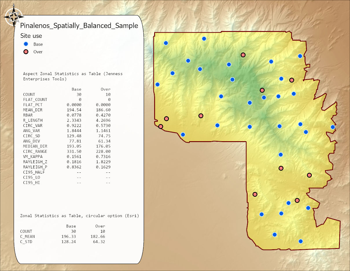
The same run shows what the extra statistics add. Both groups of points face south on average, but the mean direction alone says nothing about how much to trust that. The Base group's mean resultant length of 0.078 and its Rayleigh p of 0.84 say the 30 points face every which way and the mean is not worth reading; the Over group's 0.427 and p of 0.16 say the ten points lean south but not decisively. Neither group has a confidence interval: with so little concentration, the standard error of the mean direction is 32° for the Over group and far more for the Base group, past the 29° limit of the interval, which is its own statement of how loosely the mean direction is known.
The larger difference is in flat cells. Esri's circular option has no notion of a cell with no direction: the −1 that Esri's own Aspect tool writes for flat ground is taken as an angle and wrapped to 359°, so every flat cell is counted as facing a degree west of north. A test raster shows the effect. Eighty cells split evenly between 10° and 350°, plus twenty flat cells, gave a C_MEAN of 359.80° and a C_STD of 8.97°, exactly the values for 100 cells with the flat ones facing 359°; with the flat cells left out, the mean is due north and the standard deviation 10.03°. On a real raster with valley floors, lakes or plateaus, the flat cells pull every zone's mean toward north and shrink its spread. To use Esri's circular option on an aspect raster, set the −1 cells to NoData first. This tool leaves them out of the statistics and reports them in FLAT_COUNT and FLAT_PCT.
Beyond the two shared statistics, this tool writes the mean resultant length, the resultant length, the circular and angular variances, the angular deviation, the median direction, the circular range, the von Mises concentration, the Rayleigh test and the 95% confidence interval of the mean direction, and it accepts D-infinity flow-direction rasters. Esri's tool needs the Spatial Analyst or Image Analyst extension; this one does not.
A tour of the dialog
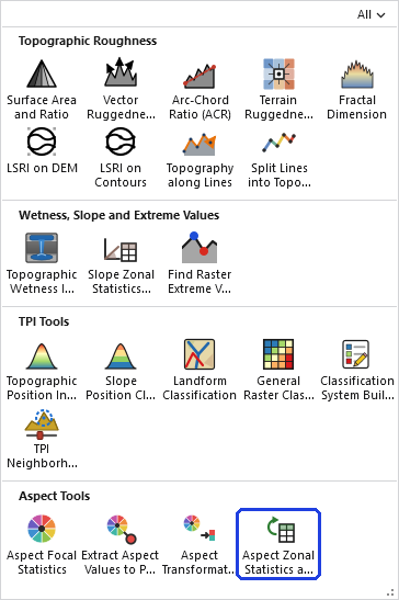
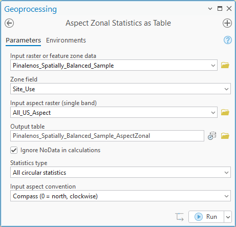
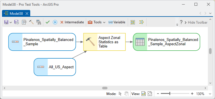
The dialog asks for the zone data and its zone field, the aspect raster, an output table, and then three options: whether to ignore NoData, which statistics to write, and the raster's direction convention. The example uses the 40 survey points in the Pinaleño Mountains from the comparison above, in their two groups, against an aspect raster of the conterminous United States.
ModelBuilder
Parameters
| Label | Explanation | Data type |
|---|---|---|
| Input raster or feature zone dataRequired · in_zone_data | The zones: an integer raster, where each distinct value is a zone, or a point, polyline or polygon feature class or layer. An active selection on a layer is honored. Overlapping features in different zones are each analyzed in full; overlapping features in the same zone count each cell once. | Feature Layer or Raster Layer |
| Zone fieldOptional · zone_field | The field defining the zones; features sharing a value form one zone. Integer, text, GUID and ObjectID fields are accepted (the ObjectID makes every feature its own zone). Required for feature zones; a zone raster always uses its cell value. | String |
| Input aspect raster (single band)Required · in_raster | The aspect raster to summarize: compass degrees 0 to 360, with −1 meaning flat, as Esri's Aspect and Surface Parameters tools produce. Any pixel type. Values outside −1 to 360 are excluded, counted and reported. D-infinity flow-direction rasters are supported through the convention setting below. | Raster Layer |
| Output tableRequired · out_table | One row per zone with the zone value, COUNT, FLAT_COUNT, FLAT_PCT and the chosen statistics. A name is suggested from the zone dataset. In a folder it becomes a dBASE .dbf, with −999 for NULL. | Table |
| Ignore NoData in calculationsOptional · ignore_nodata | Checked (the default): NoData cells within a zone are skipped. Unchecked: any zone containing a NoData cell receives NULL statistics. | Boolean |
| Statistics typeOptional · statistics_type | All circular statistics (the default), Mean Direction, Mean Resultant Length (r-bar), Resultant Length, Circular Variance, Angular Variance, Circular Standard Deviation, Angular Deviation, Median Direction, Circular Range, von Mises Concentration (kappa), Rayleigh Test (Z and p) or Mean Direction 95% Confidence Interval. COUNT, FLAT_COUNT and FLAT_PCT are always written. | String |
| Input aspect conventionRequired · input_convention | Compass (0 = north, clockwise), the default, or Mathematical (0 = east, counter-clockwise; e.g. D-infinity). Set from the raster's geoprocessing history when possible, otherwise Compass. Affects only the direction-valued outputs. | String |
Python
import arcpy
arcpy.ImportToolbox(r"C:\path\to\JennessEnterprisesTools.pyt")  # your install path
# Summarize an aspect raster by watershed polygons: all circular statistics.
arcpy.jenness.AspectZonalStatisticsAsTable(
    in_zone_data=r"C:\data\project.gdb\watersheds",
    zone_field="WSHED_ID",
    in_raster=r"C:\data\project.gdb\aspect",
    out_table=r"C:\data\project.gdb\watersheds_AspectZonal",
    ignore_nodata=True,
    statistics_type="All circular statistics",
    input_convention="Compass (0 = north, clockwise)")
# The other input_convention string:
# "Mathematical (0 = east, counter-clockwise; e.g. D-infinity)".
# Other statistics_type strings: "Mean Direction",
# "Mean Resultant Length (r-bar)", "Resultant Length", "Circular Variance",
# "Angular Variance", "Circular Standard Deviation", "Angular Deviation",
# "Median Direction", "Circular Range", "von Mises Concentration (kappa)",
# "Rayleigh Test (Z and p)", "Mean Direction 95% Confidence Interval".
Recommended citation
Credits and references
By Jeff Jenness, Jenness Enterprises (www.jennessent.com). The tool is modeled on Esri's Zonal Statistics as Table; the circular statistics follow the sources below.
- Batschelet, E. 1981. Circular Statistics in Biology. Academic Press, London. ISBN 0-12-081050-6.
- Best, D. J., and N. I. Fisher. 1981. The bias of the maximum likelihood estimators of the von Mises-Fisher concentration parameters. Communications in Statistics – Simulation and Computation 10:493–502. doi.org/10.1080/03610918108812225
- Esri. Zonal Statistics as Table (Spatial Analyst). ArcGIS Pro tool reference. doc.esri.com/en/arcgis-pro/latest/tool-reference/spatial-analyst/zonal-statistics-as-table.html. Accessed on 28 September 2026.
- Fisher, N. I. 1993. Statistical Analysis of Circular Data. Cambridge University Press, Cambridge. doi.org/10.1017/CBO9780511564345
- Greenwood, J. A., and D. Durand. 1955. The distribution of length and components of the sum of n random unit vectors. Annals of Mathematical Statistics 26:233–246. doi.org/10.1214/aoms/1177728540
- Jenness, J. 2012. Issues with directional data. Remotely Wild, newsletter of the Spatial Ecology and Telemetry Working Group of The Wildlife Society. PDF
- Mardia, K. V., and P. E. Jupp. 2000. Directional Statistics. Wiley, Chichester. doi.org/10.1002/9780470316979
- Zar, J. H. 1999. Biostatistical Analysis, 4th edition. Prentice Hall, Upper Saddle River, New Jersey. (Chapter 27, circular statistics; equation 27.4, the Rayleigh test p value.)
Licensing information
Works at every ArcGIS Pro license level (Basic, Standard, Advanced). No extension licenses are required; the zonal statistics are computed internally, without Spatial Analyst or Image Analyst.
Related tools and pages
- Slope Zonal Statistics as Table — the same zonal machinery for slope rasters, with the statistics computed on slope angles.
- Aspect Transformation — turns aspect into linear variables, such as northness and eastness, for use in ordinary statistics.
- Slope Graphic — a visual summary of slope statistics.
- Polar Plots — circular plots and the same circular statistics for directional data.
- Aspect Focal Statistics — circular statistics in a moving window rather than within zones.
- Extract Aspect Values to Points — aspect at point locations, interpolated as directions.
- About Aspect — why aspect matters, and the circular statistics behind every number in the table.