About Aspect and Circular Statistics

Topographic Analysis · Aspect Tools · concepts and circular statistics · by Jeff Jenness

What it is for

Aspect is the compass direction a slope faces: the azimuth of the steepest downhill line from a cell, measured clockwise from north, so that 0° is north, 90° east, 180° south, 270° west, and 360° is north again. A cell with no slope faces nowhere, and an aspect raster records it as −1, the flat value. Every tool on these pages reads aspect rasters made with Esri's own tools; this suite does not make them.

Aspect has a long history as a habitat variable because the two sides of a hill are different places. In the northern hemisphere a north-facing slope is typically cooler and more mesic, a south-facing slope warmer and more xeric, and the vegetation and the animals that use it can differ dramatically depending on which side of the hill you stand on (Jenness 2012). Aspect is the simplest way to put that difference on a map.

What aspect stands in for

Often the underlying driver of the differences between slopes that face different directions is solar energy, and the amount of direct sunlight a slope receives depends on aspect together with its steepness, the shading of the surrounding terrain, atmospheric conditions and the reflectivity of the ground. Where received sunlight is the real variable of interest, estimating solar insolation directly, for example with Esri's Solar Radiation tools, often captures the ecological signal better than aspect alone.

In other settings the driver is exposure to wind or water rather than to the sun. Wind scours snow from exposed windward slopes and piles it in drifts on sheltered lee slopes (Purves et al. 1998; Winstral et al. 2002). At an arctic site in the Brooks Range foothills of Alaska, where winter winds blow mostly from the south, the deepest snow lies on the steeper north-facing slopes, and plant communities dominated by Cassiope tetragona follow the deep snow (Evans et al. 1989). Wind moves more than snow. Plant litter is stripped from exposed hills and ridges and collects in drifts, where it cools the soil and adds carbon and nitrogen (Fahnestock et al. 2000). Windblown insects collect on snow patches in the lee of alpine crests, where they become a food source for alpine animals (Antor 1994). Fresh volcanic ash blew away faster from exposed and windward sites than from sheltered, concave leeward sites (Panebianco et al. 2017), and in western Wisconsin, Late Pleistocene loess is thickest on the east-southeastern flanks of bedrock ridges, downwind of the prevailing west-northwesterly winds (Schaetzl et al. 2018). On the sea floor, aspect reflects a site's exposure to currents, which may matter for suspension-feeding animals that rely on the currents to bring their food (Wilson et al. 2007).

Aspect remains valuable because it is simple, fast, and a good predictor in many settings; it just helps to know that it is a surrogate.

Why direction is different

Direction is awkward to analyze because it goes around in a circle. The difference between 0° and 359° is the same as the difference between 0° and 1°: one degree. The number line of ordinary statistics has two ends; the compass has none. Take the simplest possible case, two cells facing just either side of north:

Two cells	Arithmetic mean	Circular mean
350° and 10°	180° (due south)	0° (due north)
359° and 1°	180° (due south)	0° (due north)

Both cells face very nearly north, and the arithmetic mean says they face due south, the one direction neither comes close to. The trap is that the arithmetic mean is sometimes right: the mean of 90° and 180° really is 135°. It is right by coincidence when the directions happen not to straddle north, and wildly wrong when they do. The ordinary standard deviation fails the same way: the two cells in the first row are 20° apart on the ground and 340 apart on the number line. Jenness (2012) reduces this to two rules that account for most mistakes with directional data:

Never calculate a mean direction with the arithmetic mean. Use the vector method below.
Convert degrees to radians before taking a sine or cosine. Nearly every piece of software assumes radians; there are 2π radians, about 6.28, in a full circle, so a program fed degrees will read a change of 2° as roughly a third of the way around the circle.

The vector mean

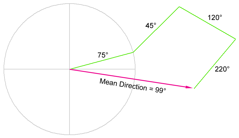
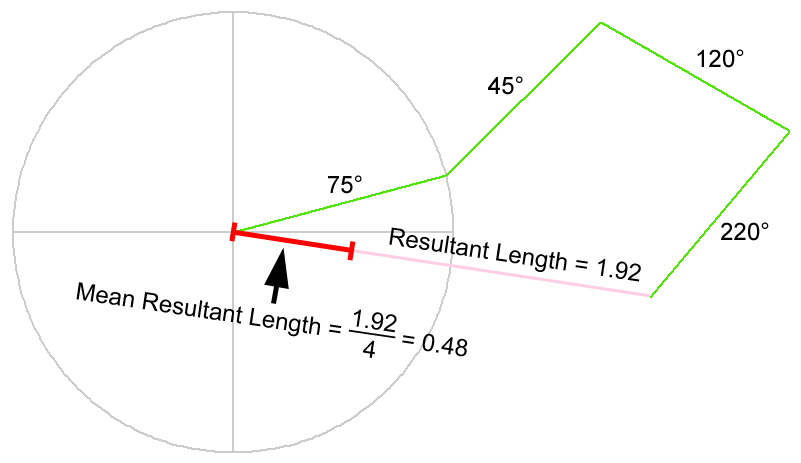
The correct method is easier to picture than to write down. Treat each direction as an arrow of length one pointing that way, and lay the arrows head to tail, in any order, as if walking a path. The mean direction is the bearing from the start of the path to its end. The mean resultant length is the straight-line distance from start to end divided by the number of arrows. If every arrow points the same way the path is straight, and the mean resultant length is 1; the more the path wanders, the shorter the straight-line distance, and if the path ends back where it began the mean resultant length is 0.

Take four directions, 45°, 75°, 120° and 220°:

A circle with four directions drawn from its center as green lines at bearings of 45, 75, 120 and 220 degrees — Four compass directions: 45°, 75°, 120° and 220°.

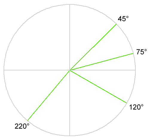
Laid head to tail, they make a path that leaves the center of the circle and ends a little south of due east of it. The bearing from the start of the path to its end is the mean direction, 99°:

The four direction arrows joined end to end into a path leaving the circle's center, with a pink arrow from the start to the end of the path labeled Mean Direction = 99 degrees — The four arrows strung end to end. The pink arrow from the start of the path to its end points in the mean direction, 99°.

The same straight line, measured instead of aimed, is the resultant. It is 1.92 units long, and dividing by the four arrows gives a mean resultant length of 0.48:

The same path, with a pink line from the start to the end of the path labeled Resultant Length = 1.92, and a red segment labeled Mean Resultant Length = 1.92 / 4 = 0.48 — The resultant is 1.92 units long; divided by the four arrows, the mean resultant length is 0.48.

The same picture describes an animal's movements. If a collar records an elk's positions through a day, the average direction it moved is simply the bearing from the first fix to the last (Jenness 2012); the fixes are the arrows, laid head to tail in the order they happened.

The circular statistics

In symbols, for n directions θ_i each treated as a unit vector with an east–west component sin θ and a north–south component cos θ:

\bar{S} = \frac{1}{n} \sum_{i = 1}^{n} \sin θ_{i} \bar{C} = \frac{1}{n} \sum_{i = 1}^{n} \cos θ_{i}

\bar{R} = \sqrt{{\bar{S}}^{2} + {\bar{C}}^{2}} \bar{θ} = atan2 (\bar{S}, \bar{C})

S̄ and C̄ are the mean sine and mean cosine, R̄ is the mean resultant length, the length of the average arrow, and θ̄ is the mean direction, the compass bearing of that arrow; atan2 is the two-argument arctangent that returns the whole 0° to 360° circle. The resultant length itself, R, is the length of the summed arrow, n times R̄. Everything else follows from these.

Important: sin θ is the east–west component and cos θ the north–south component only when θ is a compass direction, with 0° at true north and values increasing clockwise, as in an aspect raster (converted to radians before the sine and cosine are taken). Directions are sometimes reported instead in mathematical polar coordinates, with 0° due east and values increasing counterclockwise; the D-infinity (DINF) option of Esri's Flow Direction tool is one example (see Flat cells and flow-direction rasters below). In that convention the roles are reversed: cos θ is the east–west component and sin θ the north–south component. The mean direction and mean resultant length still come out right in either convention, as long as every direction uses the same one; only the reading of the two components changes, and a mean direction computed in the mathematical convention must be converted before it is read as a compass bearing.

A worked example

Five cells of a hillside that faces roughly north, three of them just east of north and two just west of it:

Aspect θ	sin θ (east–west)	cos θ (north–south)
340°	−0.3420	0.9397
355°	−0.0872	0.9962
5°	0.0872	0.9962
20°	0.3420	0.9397
30°	0.5000	0.8660
Mean	S̄ = 0.1000	C̄ = 0.9476

The mean arrow points a little east of north: its direction is atan2(0.1000, 0.9476) = 6.0°, and its length is R̄ = 0.953, close to 1, because the five cells agree closely. The arithmetic mean of the same five numbers is 150°, roughly south-southeast. That answer is not a little off; it is wrong by 144°, pointing to nearly the opposite side of the hill. Every one of the five cells faces within 30° of north, and the arithmetic mean puts their average in a direction that none of them comes anywhere near. A habitat model given that number would treat this cool, north-facing slope as though it faced the warm, dry side of the hill.

Dispersion and concentration

Mardia and Jupp (2000), Fisher (1993) and Batschelet (1981) describe several measures of spread, all built on R̄ and all zero when every direction is the same. Two are variances and two are deviations. The angular deviation is the square root of the angular variance, but the circular standard deviation is defined on its own, from the logarithm of R̄, and is not the square root of the circular variance. The deviations come out in radians and are converted to degrees for reporting:

V = 1 - \bar{R} s^{2} = 2 (1 - \bar{R})

v = \sqrt{- 2 \ln \bar{R}} s = \sqrt{2 (1 - \bar{R})}

V is the circular variance and v the circular standard deviation (Mardia and Jupp 2000; Fisher 1993); s² is the angular variance and s the angular deviation (Batschelet 1981). For the five cells above, V is 0.047, the circular standard deviation 17.8° and the angular deviation 17.6°. The two deviations agree when the directions are concentrated and part company as they spread: the circular standard deviation grows without limit as R̄ approaches 0, which makes it the closer analog of an ordinary standard deviation for tightly grouped data.

The angular deviation, in contrast, stays constrained. It can never exceed √2 radians, about 81°, however scattered the directions are. Batschelet (1981, p. 278) notes that it remains finite as the mean resultant length approaches 0, while the circular standard deviation tends to infinity, “which is somewhat strange for a finite distribution.” Batschelet (1981, pp. 34–35) also reproduces a geometric construction of the angular deviation, credited to Seyfarth and Barth (1972), that shows what it means:

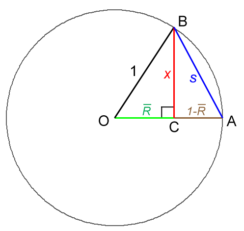
A unit circle centered on O. Point A lies on the circle due right of O. Point C lies on segment OA at distance R-bar from O, leaving 1 minus R-bar from C to A. Point B lies on the circle directly above C, joined to O by a radius of length 1. The vertical segment BC is labeled x, and the segment from B to A is labeled s, the angular deviation. — The angular deviation s as the distance from A to B on a unit circle, with C placed R̄ along OA.

On a circle of radius 1, put point A on the circle due right of the center O, point C a distance R̄ along OA (R̄ is always between 0 and 1), and point B on the circle directly above C. The angular deviation s is the length of the line from A to B. The Pythagorean theorem on triangle BCO, and then on triangle ABC, gives it (colors match the figure):

From the Pythagorean theorem on triangle BCO:

\begin{matrix} x^{2} + {\bar{R}}^{2} & = 1^{2} \\ ∴ x^{2} & = 1 - {\bar{R}}^{2} \end{matrix}

From the Pythagorean theorem on triangle ABC:

\begin{matrix} s^{2} & = {(1 - \bar{R})}^{2} + x^{2} \end{matrix}

Substituting for x²:

\begin{matrix} s^{2} & = {(1 - \bar{R})}^{2} + (1 - {\bar{R}}^{2}) \\ = (1 - \bar{R}) (1 - \bar{R}) + 1 - {\bar{R}}^{2} \\ = 1 - 2 \bar{R} + {\bar{R}}^{2} + 1 - {\bar{R}}^{2} \\ = 2 - 2 \bar{R} \\ = 2 (1 - \bar{R}) \\ ∴ s & = \sqrt{2 (1 - \bar{R})} \end{matrix}

When the directions all agree, R̄ = 1, C sits on A, and s = 0. When they cancel completely, R̄ = 0, C sits on the center, and s is the chord from A to the top of the circle, √2 radians (81.03°), the largest value it can take. Batschelet adds one caution: the construction draws s as a straight line, but conceptually it is the length of an arc.

Three more statistics describe a set of directions from other angles. The median direction is the observed direction with the least total circular distance to all the others, a center that is less swayed by a few outlying cells than the mean. The circular range is the smallest arc that contains every direction, 360° minus the largest empty gap; for the five cells it is 50°, from 340° round to 30°. The von Mises concentration κ is the parameter of the von Mises distribution, the circular counterpart of the normal distribution, estimated from R̄ by the piecewise approximation of Best and Fisher (1981, p. 495), also given by Fisher (1993, equation 4.40): 0 for directions spread uniformly around the circle, larger the more they cluster. Best and Fisher showed that in a small sample the estimate runs too high, by a considerable amount, and proposed a corrected estimator (p. 498); Fisher (1993, equation 4.41) recommends it for 15 or fewer directions, and the tools apply it there. The five cells give 10.9 before the correction and 5.35 after it.

Is there a preferred direction at all?

The Rayleigh test asks whether a set of directions has any preferred direction. Its null hypothesis is that they are spread uniformly around the circle, and a small p says they face somewhere in particular. The tools use Zar's (1999) equation 27.4, which with R = nR̄ is

p = \exp [\sqrt{1 + 4 n + 4 (n^{2} - R^{2})} - (1 + 2 n)]

For the five cells, p = 0.0041. The 95% confidence interval of the mean direction uses the von Mises standard error, 1 / √(n R̄ κ), and a half-angle equal to the arcsine of 1.96 times that (Fisher 1993, equations 4.42 and 4.43); for the five cells it is ±22.8°, so the mean of 6° is bracketed by 343.2° and 28.9°. The half-angle is an arcsine, and an arcsine exists only for values up to 1, so the interval exists only while the standard error of the mean direction is less than 1 / 1.96, about 0.51 radians or 29°. Beyond that the directions are too dispersed for an interval, and none is reported. Fisher (1993, Table 4.3) recommends this interval only when the concentration is strong enough for the sample size: for any sample when κ is 2 or more, for at least 10 directions when κ is between 1.5 and 2, at least 15 when it is between 1 and 1.5, and at least 25 when it is between 0.4 and 1. Below 0.4 he advises a bootstrap interval instead, whatever the sample size. The tools compute the interval outside that range too, and warn that they have.

Both the test and the interval assume the directions are independent observations, which neighboring raster cells are not. That is almost always the case in zonal statistics when the zones come from a categorical raster or from polygons or polylines, since every zone is a block of neighboring cells; there the test and the interval are best read as lower bounds. Point zones can be different. Points that were generated or selected to be independent, such as randomly placed sample locations or survey plots spread farther apart than the distance over which aspects stay similar, may well be independent enough that the test and the interval mean what they say. Points crowded close together, such as animal locations recorded minutes apart, share the cells' autocorrelation, and the same caution applies. The Aspect Zonal Statistics as Table page discusses both cases, and the Slope Zonal Statistics as Table page shows how far the correlation between cells reaches on a real slope raster: the slopes of cells 2.8 km apart are still correlated.

Reading the mean resultant length

The mean resultant length is the single most useful number in any of these tables, but it has to be read with care. A value near 1 always means the same thing: the directions are tightly focused. A value near 0 does not mean the opposite. It means only that the arrows cancel, and they can cancel in two very different ways. Directions scattered evenly around the compass cancel, and that is genuine dispersion. So do directions split between two opposite bearings. Jenness (2012) gives the example of a bird with separate roost and foraging sites that flies out each morning and back each evening: its movement directions are about as focused and predictable as movement can be, yet its mean resultant length is 0 and its circular variance is at the maximum. On the ground, a symmetric valley whose walls face east and west does the same thing. So read a mean direction only when R̄ is well above 0; when it is near 0, the mean direction is the bearing of an arrow with almost no length, and it is worth looking at the data themselves to see whether the directions truly go every which way or are tightly focused in opposing groups, like the bird's two headings. That is a good habit in general: always look at the data, not only at the statistics computed from them. A polar plot of the directions, or a glance at the aspect raster itself, often shows at once what a single number hides.

Turning aspect into a number

Circular statistics describe a set of directions. Using aspect as a predictor in an ordinary statistical model or a habitat score is a different problem, because the raw angle cannot go into a regression as it stands. Jenness (2012) describes three routes, each with a cost:

Classes. Group the angles into a few named directions, such as North 315° to 45°, East 45° to 135°, South 135° to 225° and West 225° to 315°, which makes a categorical variable suited to some analyses. The Aspect Transformation tool produces the standard two-, four- and eight-direction classes. For any other scheme, write the classes in the Classification System Builder and apply them with the General Raster Classification tool. A North class that wraps past 360° takes two conditions joined by OR (greater than 315, or at most 45), and a Flat class for Esri's −1 value, given a lower class value than North so that it takes precedence, keeps flat cells out of North.
Deviation from a bearing. Express each aspect as its angular distance, 0° to 180°, from a direction of interest, such as deviation from north where the north-versus- south contrast is the point. The interval stays constant: one degree is one degree everywhere on the scale.
Sine and cosine. Decompose the angle into an east–west component, the sine, which runs from −1 at due west to 1 at due east, and a north–south component, the cosine, from −1 at due south to 1 at due north (after converting to radians). The interval is not constant: the sine changes by 0.00015 between 90° and 91° and by 0.017 between 180° and 181°, more than two orders of magnitude, which matters for a method that assumes interval-level data.

A fourth route is the cosine of the deviation from a chosen bearing, which scores 1 facing that bearing, 0 at right angles to it and −1 facing away. Trimble and Weitzman (1956) introduced it in site-productivity research, with the maximum placed at the northeast, 45°, where the best upland oaks of their study grew, and Beers, Dress and Wensel (1966) generalized it to any optimum bearing. The Aspect Transformation tool writes all of these.

Flat cells and flow-direction rasters

A flat cell has no direction, and no statistic can be computed from it, so the tools exclude flat cells (−1) from every statistic but count them, reporting how many there were, and give an all-flat neighborhood or zone a defined result rather than a misleading one. In the transformation tool the trigonometric outputs are NoData at flat cells, because −1 would look like a real value there: due south for northness, due west for eastness.

A D-infinity flow-direction raster is essentially an aspect raster, since it records the direction of steepest descent, but in the mathematical convention, 0 = east and increasing counter-clockwise, rather than the compass convention of an aspect raster. Every aspect tool has an Input aspect convention setting for it, and suggests the setting when it recognizes a D-infinity raster. The dispersion, concentration and test statistics are identical under either convention, since they do not care where 0 sits or which way angles turn; only the mean and median direction differ, and the tools convert those to compass. A standard D8 flow-direction raster stores codes 1 to 128, not degrees, and is not a direction raster at all.

The four tools at a glance

Each tool is the circular counterpart of a standard Esri tool, built for aspect. None needs the Spatial Analyst extension.

Tool	What it does
Aspect Focal Statistics	Circular statistics over a neighborhood, one statistic per run, with the same neighborhood shapes as Esri's Focal Statistics: mean and median direction, the dispersion and concentration measures, the Rayleigh test and the proportion of cells with a defined aspect.
Extract Aspect Values to Points	The aspect at each point, as Esri's Extract Values to Points does, with the optional interpolation done as a weighted mean direction rather than a linear average.
Aspect Transformation	Direction classes, northness, eastness, and the deviation from a bearing, several at once.
Aspect Zonal Statistics as Table	Circular statistics per zone, as Esri's Zonal Statistics as Table does for ordinary rasters.

The Polar Plots window, under Terrain Graphs, draws the distribution of a set of directions as a rose diagram and the other circular plots, which is usually the first thing to do with directional data before computing anything.

Credits and references

By Jeff Jenness, Jenness Enterprises (www.jennessent.com). The discussion follows his 2012 newsletter article on directional data; the statistics follow the standard texts listed here.

Antor, R. J. 1994. Arthropod fallout on high alpine snow patches of the Central Pyrenees, northeastern Spain. Arctic and Alpine Research 26:72–76. doi.org/10.1080/00040851.1994.12003042
Batschelet, E. 1981. Circular Statistics in Biology. Academic Press, London. ISBN 0-12-081050-6.
Beers, T. W., P. E. Dress, and L. C. Wensel. 1966. Aspect transformation in site productivity research. Journal of Forestry 64:691–692. doi.org/10.1093/jof/64.10.691
Best, D. J., and N. I. Fisher. 1981. The bias of the maximum likelihood estimators of the von Mises-Fisher concentration parameters. Communications in Statistics – Simulation and Computation 10:493–502. doi.org/10.1080/03610918108812225
Evans, B. M., D. A. Walker, C. S. Benson, E. A. Nordstrand, and G. W. Petersen. 1989. Spatial interrelationships between terrain, snow distribution and vegetation patterns at an arctic foothills site in Alaska. Holarctic Ecology 12:270–278. doi.org/10.1111/j.1600-0587.1989.tb00846.x
Fahnestock, J. T., K. L. Povirk, and J. M. Welker. 2000. Ecological significance of litter redistribution by wind and snow in arctic landscapes. Ecography 23:623–631. doi.org/10.1111/j.1600-0587.2000.tb00181.x
Fisher, N. I. 1993. Statistical Analysis of Circular Data. Cambridge University Press, Cambridge. doi.org/10.1017/CBO9780511564345
Jenness, J. 2012. Issues with directional data. Remotely Wild, newsletter of the Spatial Ecology and Telemetry Working Group of The Wildlife Society. PDF
Mardia, K. V., and P. E. Jupp. 2000. Directional Statistics. Wiley, Chichester. doi.org/10.1002/9780470316979
Panebianco, J. E., M. J. Mendez, D. E. Buschiazzo, D. Bran, and J. J. Gaitán. 2017. Dynamics of volcanic ash remobilisation by wind through the Patagonian steppe after the eruption of Cordón Caulle, 2011. Scientific Reports 7:45529. doi.org/10.1038/srep45529
Purves, R. S., J. S. Barton, W. A. Mackaness, and D. E. Sugden. 1998. The development of a rule-based spatial model of wind transport and deposition of snow. Annals of Glaciology 26:197–202. doi.org/10.3189/1998AoG26-1-197-202
Schaetzl, R. J., P. H. Larson, D. J. Faulkner, G. L. Running, H. M. Jol, and T. M. Rittenour. 2018. Eolian sand and loess deposits indicate west-northwest paleowinds during the Late Pleistocene in western Wisconsin, USA. Quaternary Research 89:769–785. doi.org/10.1017/qua.2017.88
Seyfarth, E.-A., and F. G. Barth. 1972. Compound slit sense organs on the spider leg: mechanoreceptors involved in kinesthetic orientation. Journal of Comparative Physiology 78:176–191. doi.org/10.1007/BF00693611
Trimble, G. R., Jr., and S. Weitzman. 1956. Site index studies of upland oaks in the northern Appalachians. Forest Science 2:162–173. doi.org/10.1093/forestscience/2.3.162
Wilson, M. F. J., B. O’Connell, C. Brown, J. C. Guinan, and A. J. Grehan. 2007. Multiscale terrain analysis of multibeam bathymetry data for habitat mapping on the continental slope. Marine Geodesy 30:3–35. doi.org/10.1080/01490410701295962
Winstral, A., K. Elder, and R. E. Davis. 2002. Spatial snow modeling of wind-redistributed snow using terrain-based parameters. Journal of Hydrometeorology 3:524–538. doi.org/10.1175/1525-7541(2002)003<0524:SSMOWR>2.0.CO;2
Zar, J. H. 1999. Biostatistical Analysis, 4th edition. Prentice Hall, Upper Saddle River, New Jersey. (Chapter 27, circular statistics; equation 27.4, the Rayleigh test p value.)

Aspect Focal Statistics
Extract Aspect Values to Points
Aspect Transformation
Aspect Zonal Statistics as Table
Polar Plots — rose diagrams and other circular plots of a set of directions, with the same statistics.
About Topographic Roughness — the neighborhood measures of how rough the terrain is; the Vector Ruggedness Measure there is a circular idea in three dimensions.
Projecting Rasters — the aspect tools handle geographic rasters correctly, but if you do project a DEM before deriving aspect, project it with bilinear interpolation.