

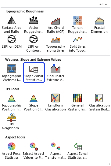
Slope Zonal Statistics as Table
Summary
Summarizes a slope raster within zones and writes the results to a table: one row per zone, holding the count of cells, the mean, median, standard deviation, minimum, maximum, range, 5th and 95th percentiles, and the 95% confidence interval of the mean slope. The zones can be an integer raster or a point, polyline or polygon feature class. The tool is deliberately modeled on Esri's Zonal Statistics as Table, and it is aimed at one kind of raster in particular: slope. Slope rasters come in degrees, percent, rise:run ratio or gradians, and the mean, standard deviation and confidence interval of a set of slopes depend on which of those units you average in. This tool converts every value to a slope angle before computing those statistics, then converts the results back to the raster's own unit for display, so the average steepness it reports is the same whatever unit the raster happens to use. No Spatial Analyst or Image Analyst extension is needed; every calculation is done internally.
Why slope statistics belong in angle space
Terrain steepness is an angle, the angle between the ground surface and the horizontal. Percent slope is a different way of writing the same steepness: it is 100 times the rise over the run, and rise over run is the tangent of the slope angle. So a percent-slope raster is a raster of tangents, multiplied by 100. That matters as soon as you average, because the tangent is not a straight-line function of the angle. It grows slowly at gentle angles and faster and faster as the angle steepens, which is what a mathematician calls a convex function. Take the mean of a set of tangents and you weight the steep cells more heavily than the gentle ones, and the average comes out too steep. Here is the classroom example: a landscape with half its cells at 50° and half at 70°.
| Cells | Slope angle | Rise over run (tangent) | Percent slope |
|---|---|---|---|
| Half the landscape | 50° | 1.1918 | 119.2% |
| The other half | 70° | 2.7475 | 274.7% |
| Mean of the angles | 60° | 1.7321 | 173.2% |
| Mean of the percents | 63.1° | 1.9696 | 197.0% |
The true average steepness of that landscape is 60°, halfway between the two. Averaging the same cells as percents gives 197%, and 197% is a 63.1° slope, three degrees too steep. The landscape did not get steeper because it was measured in a different unit; the arithmetic did that. The size of the bias depends on how steep and how varied the slopes are. For two cells at the angles shown, the mean of their tangents converts back to these angles:
| Two slopes | Mean of the angles | Angle of the mean tangent | Bias |
|---|---|---|---|
| 10° and 20° | 15.0° | 15.1° | +0.1° |
| 30° and 50° | 40.0° | 41.5° | +1.5° |
| 50° and 70° | 60.0° | 63.1° | +3.1° |
| 60° and 80° | 70.0° | 74.9° | +4.9° |
| 70° and 89° | 79.5° | 88.1° | +8.6° |
On gentle ground the two answers are nearly the same, because the tangent is nearly a straight line near zero. On steep, varied ground they part company, and the bias is always in the same direction: too steep. The last row shows how fast it grows near vertical: the tangent of 70° is 2.75, a slope of 275%, but the tangent of 89° is 57.3, a slope of 5,729%, so the steeper cell swamps the mean of the percents, which converts back to 88.1°, 8.6° steeper than the true average. The Terrain Ruggedness Index page shows the same tangent curve from the other side, where its runaway growth toward vertical is a feature of a ruggedness score, and in that case the increasing weight of steep slopes is put to work to help identify exceptionally rugged landscapes. For this tool, however, the goal is the true statistical properties of the slopes in a landscape, so the calculation takes care to average them the correct way.
So this tool computes its statistics in angle space. Every input value passes through the arctangent (or, for gradians, a simple rescaling) to become a slope angle in degrees. The mean, the standard deviation and the confidence interval are then computed on those angles. The mean is converted back to the raster's unit for display: the reported mean of a percent-slope raster is the tangent of the mean angle, times 100, never the mean of the tangents. The median, the 5th and 95th percentiles, the minimum, the maximum and the range are order statistics: they pick out particular cells rather than averaging, and because converting a value to an angle never changes which cell is steeper than which, they are identical whether you compute them in percent or in degrees. The minimum and maximum are exact cell values; the median and the two percentiles are read from a histogram of 0.02° bins, so they are bin centers, accurate to ±0.01°. Only the moment statistics, the mean, standard deviation and confidence interval, are affected by the unit, and those are the ones done on angles.
Two of the outputs are reported in degrees no matter what unit the raster uses: the standard deviation and the half-width of the confidence interval. A single value, such as a mean of 35°, converts exactly to a percent (70%). A dispersion does not. A standard deviation of 10° around a mean of 35° spans 25° to 45°, which is 47% to 100%, and there is no single percent value that expresses that spread without misrepresenting it. The tool therefore leaves the standard deviation and the confidence-interval half-width in degrees, and it gives the confidence interval's lower and upper bounds, which are single values, in the raster's unit.
Units and how they are detected
The Slope units of the input raster drop-down names the unit the raster's values are in. There are four choices:
- Degrees (-90 to 90): the slope angle itself.
- Percent slope (rise/run × 100): also called grade; 45° is 100%, and there is no upper limit.
- Rise:run ratio: the tangent itself, percent divided by 100; again no upper limit.
- Gradians (gons): a right angle divided into 100 parts, so 100 gon is 90°.
The tool fills this in for you when it can. Esri's Slope and Surface Parameters tools record their output unit (DEGREE or PERCENT_RISE) in the geoprocessing history stored in the raster's metadata, and the tool reads that history when you pick a raster and sets the drop-down to match. When the history says nothing, the drop-down falls back to Degrees. Always check it: a percent raster treated as degrees, or the reverse, gives statistics that are simply wrong.
Values outside the valid range for the chosen unit are excluded from the statistics and, for raster, polygon and polyline zones, counted and reported with a warning that the raster might not be a slope raster in that unit. At point zones such a cell is left out of the interpolation, and the warning counts the points that lost a neighboring cell that way and any left with no value at all. For degrees the valid range is −90 to 90; for gradians, −100 to 100. Percent and ratio are unbounded, so nothing is excluded on those grounds.
Signed slopes
Most slope rasters hold only positive values, but some are signed: the pitch along a road or a trail, for example, where uphill is positive and downhill negative. The Treat negative slopes as positive option, checked by default, takes the absolute value of every cell first, so the statistics describe absolute steepness, how steep the ground is regardless of which way it faces. Unchecked, values keep their sign, and a downhill cell can cancel an uphill one in the mean, which is what you want for signed directional data and not what you want for terrain. Either way, the output table reports how many cells in each zone were negative in the source, in the NEG_COUNT field, so signed data always announces itself.
Zones
Zones can come from an integer raster, in which case every distinct cell value is a zone, or from a point, polyline or polygon feature class or layer, in which case all features sharing the same value in the Zone field form one zone. A zone raster must be an integer raster in the same coordinate system as the slope raster. Integer, text, GUID and ObjectID fields are all valid zone fields; choosing the ObjectID makes every feature its own zone. An active selection on a layer is honored.
A feature layer with a table joined to it works too: the joined fields appear in the zone-field list under their qualified names, such as lookup.Unit, and any of them can define the zones. A raster zone always uses its cell values, so the zone field for a zone raster is always Value.
Feature zones are processed one zone at a time, each over its own window of the slope raster, so zones that overlap are each analyzed in full, and within a single zone, features that overlap each other count each cell once. That was a long-standing problem in earlier versions of Esri's zonal tools, which rasterized the zones first, so that one of two overlapping polygons silently lost the cells they shared. The current Esri tool no longer does this: its documentation says that overlapping features are each analyzed individually, and in a test in ArcGIS Pro 3.7 it gave the same counts and means as this tool for overlapping zones and for overlapping features of one zone.
How a feature claims cells depends on its geometry:
- Polygons use every cell whose center falls inside the polygon.
- Polylines use every cell the line passes through.
- Points take the slope at the point itself, interpolated bilinearly from the four surrounding cell centers, with the interpolation done on the slope angles. A NoData cell among the four is dropped and the weights of the rest are renormalized; a point whose four cells are all NoData gets no value.
Only the part of the raster under the zones is read, and the tool's large-raster check applies to that part rather than to the whole raster, so a statewide slope raster and a few small zones make a quick run.
Zones that lie entirely outside the raster do not appear in the output table, which matches the Esri tool's behavior of working on the intersection of the extents. Polygons stored with true curves, such as the circles a geodatabase Buffer produces, are densified automatically before their cells are gathered, so a circular plot yields its full complement of cells. If Ignore NoData in calculations is unchecked, any zone that contains even one NoData cell receives NULL statistics, again matching the Esri tool with the same setting; checked, which is the default, NoData cells are simply skipped.
The output table
The table has one row per zone. Its fields, in order, are the zone value (named after the zone field), COUNT (the number of cells used, or of points for point zones), NEG_COUNT (the number of values that were negative in the source), and then whichever statistics were requested:
| Field | What it holds | Unit |
|---|---|---|
| MEAN | The mean slope, computed on the angles and converted back. | Source unit |
| MEDIAN | The middle value. | Source unit |
| SD_DEG | The standard deviation of the slope angles. | Degrees |
| MIN, MAX, RANGE | The least and greatest values, and their difference. | Source unit |
| P05, P95 | The 5th and 95th percentiles. | Source unit |
| CI95_HALF_DEG | Half the width of the 95% confidence interval of the mean angle. | Degrees |
| CI95_LO, CI95_HI | The lower and upper bounds of that interval, converted back. | Source unit |
The 95% confidence interval of the mean uses the t distribution (Zar 1999, chapter 7), with the exact t value for the zone's sample size. The confidence interval says how well the mean is known, not how variable the slopes are; the standard deviation answers the second question.
| Distance between two cells | 1 cell (28 m) | 5 cells (141 m) | 20 cells (565 m) | 100 cells (2.8 km) |
|---|---|---|---|---|
| Correlation of their slopes | 0.96 | 0.79 | 0.56 | 0.29 |
Treat the interval with care when the zones come from an integer raster or from polygons or polylines. Like every t interval, it assumes that each value is an independent observation, and neighboring raster cells are nothing of the kind. The table shows how strongly the slope of one cell predicts the slope of another on the Coconino slope raster used in the example below: even cells 2.8 km apart are still correlated. Part of that is the terrain itself, and part is the slope calculation, since the 3 × 3 windows of two adjacent cells share six cells, four of which Horn's method uses for both slopes. A zone of 100,000 correlated cells carries far less independent information than 100,000 separate measurements, so the interval the tool reports is much narrower than the real uncertainty of the mean, and it should be read as a lower bound, useful mainly for comparing zones of similar size. There is a more basic point as well. When a zone's cells are all the cells in that zone, the tool has taken a census rather than a sample, and the mean slope of the zone is simply known, apart from errors in the DEM; an interval becomes meaningful only when the cells are treated as a sample of some larger process, and then the autocorrelation has to be taken into account by other means.
Point zones are a different case. Each point contributes a single interpolated value, and points spread farther apart than the distance over which slopes stay correlated, such as survey plots or randomly placed sample locations, can well be independent observations. For points like those, the confidence interval means what it says. A zone with a single point has no standard deviation and no interval, and a zone whose points all have the same slope has a standard deviation of zero and no interval; those fields are NULL (−999 in a dBASE table). Points crowded close together, such as animal locations recorded minutes apart, share the same autocorrelation as the cells, and the same caution applies.
A table written to a folder rather than a geodatabase becomes a dBASE table. The tool adds the .dbf extension, shortens CI95_HALF_DEG to CI95_HALF because dBASE field names are limited to ten characters, and writes −999 for any statistic it cannot compute for a zone, because a dBASE table cannot hold a NULL. The output table's metadata records the inputs and settings that produced it, and the tool prints a ready-to-run Python snippet in its messages so the run can be repeated in a script.
A tour of the dialog
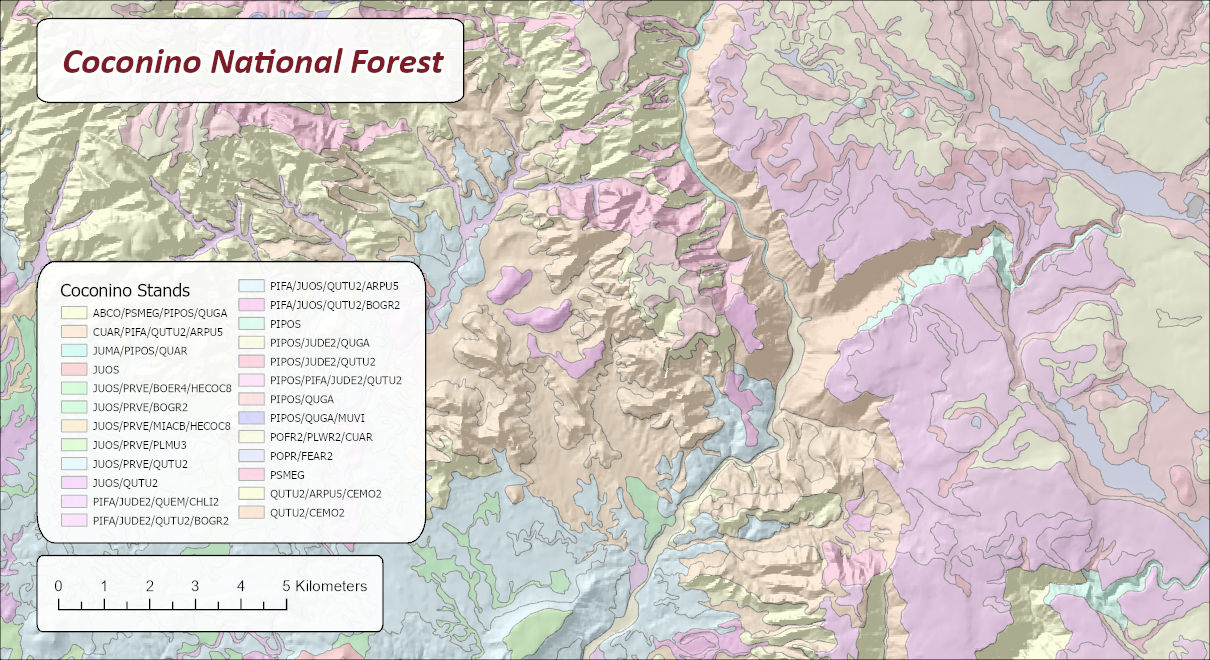
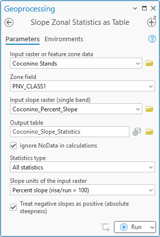
The example asks whether the potential natural vegetation types of the Coconino National Forest, near Flagstaff, Arizona, differ in how steep the ground under them is. Potential natural vegetation is the plant community a site would support if succession ran its course without disturbance, as distinct from the vegetation growing there today. The polygons, in a layer named Coconino Stands, are the landtype map units of the Forest Service's Terrestrial Ecological Unit Inventory, and each carries its most dominant potential natural vegetation type in the field PNV_CLASS1. The statistics are wanted by vegetation type, not by individual polygon, so PNV_CLASS1 is the zone field: every polygon of one type, wherever it lies on the forest, falls in the same zone. The 5,966 polygons fall into 75 types. The slope raster is percent slope with cells of about 28 m. The type names are strings of USDA PLANTS database symbols, the Forest Service's standard plant codes, listed from the most dominant species: PIPOS/QUGA is ponderosa pine with Gambel oak, and any code can be looked up in the PLANTS database.
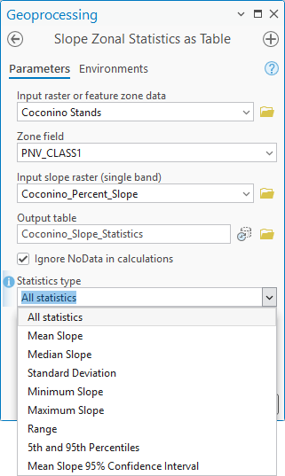
The dialog asks for the zone data and its zone field, the slope raster, an output table, and then the four options: whether to ignore NoData, which statistics to write, the raster's unit, and whether to take absolute values.
The run takes about 15 seconds on this data: the polygons are rasterized one vegetation type at a time onto the slope raster's grid, and the messages report each type as it finishes, with its number of polygons, its number of cells and the time it took.
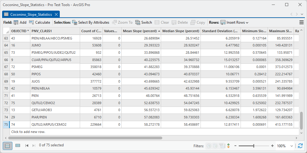
The answer to the question is plain in the table. Across the 75 potential natural vegetation types the mean slope runs from 1.1% (CAAQ/ELMA3/POLA4/ALGE) to 58.3% (QUTU2/ARPU5/CEMO2), so the types differ very strongly in the ground they occupy. The most extensive type, PIPOS/QUGA, with more than two million cells, averages 9.4%.
Sorted by mean slope, the types fall into bands that follow the vegetation of the region. The nearly level ground, 1% to 6%, holds a wet meadow of water sedge at 1.1%, the grasslands of blue grama, Arizona fescue and wheatgrass, open pinyon-juniper grassland, and velvet mesquite and creosote bush desert. The ponderosa pine types sit on gentle ground, mostly 5% to 11%. Pinyon-juniper and pine types with a shrub layer of cliffrose, Apache plume or scrub oak, mixed conifer, and the riparian cottonwood and sycamore types run from about 10% to 25%. Engelmann spruce, corkbark fir and Douglas-fir occupy steeper ground, 24% to 48%, as do all five types named by a single species (oneseed juniper, Douglas-fir, ponderosa pine, Utah juniper and Engelmann spruce, 29% to 48%). The steepest ground of all, 52% to 58%, belongs to the Sonoran scrub oak and manzanita chaparral and to the alpine and bristlecone pine types of the San Francisco Peaks. The pattern is a description of where each type occurs on this forest, not a test of why; slope travels with elevation, soils and aspect, and the table alone cannot separate them.
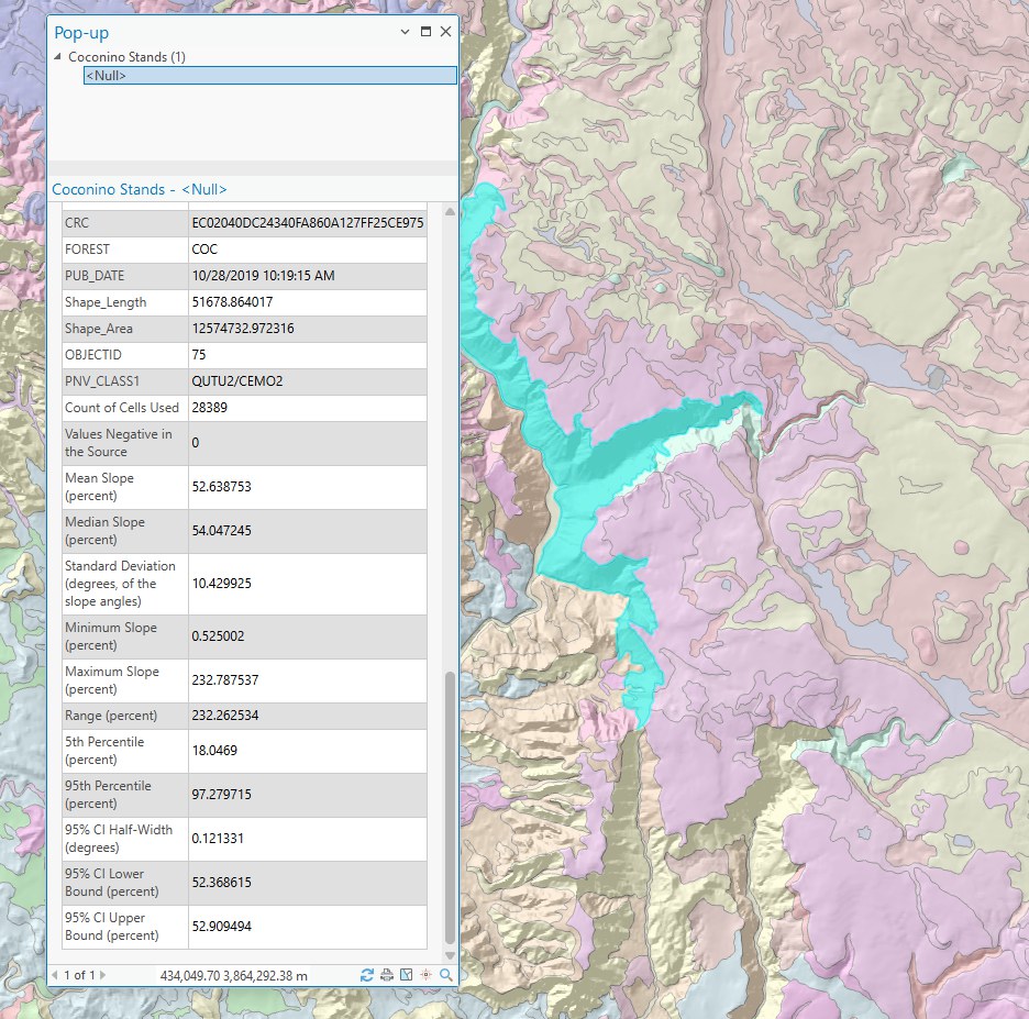
Because the table has one row per vegetation type, keyed by the same PNV_CLASS1 values as the polygons, it can be joined back to the feature class with Add Join, joining PNV_CLASS1 in the polygons to PNV_CLASS1 in the table. Every polygon then carries the statistics of its type, so clicking any polygon shows how steep its type is across the whole forest, and the polygons can be symbolized by the mean slope of their type.
The same run works on a slope raster in degrees, in rise:run ratio or in gradians: choose the unit in the Slope units drop-down, or let the tool read it from the raster's history. Because the statistics are computed on slope angles whatever the unit, a degree raster and a percent raster of the same ground give the same answers: the percent table's MEAN is the tangent of the degree table's MEAN, times 100, and SD_DEG is identical in both.
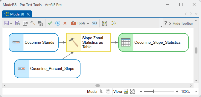
ModelBuilder
Parameters
| Label | Explanation | Data type |
|---|---|---|
| Input raster or feature zone dataRequired · in_zone_data | The zones: an integer raster, where each distinct value is a zone, or a point, polyline or polygon feature class or layer. An active selection on a layer is honored. Overlapping features in different zones are each analyzed in full; overlapping features in the same zone count each cell once. | Feature Layer or Raster Layer |
| Zone fieldOptional · zone_field | The field defining the zones; features sharing a value form one zone. Integer, text, GUID and ObjectID fields are accepted (the ObjectID makes every feature its own zone). Required for feature zones; a zone raster always uses its cell value. | String |
| Input slope raster (single band)Required · in_raster | The slope raster to summarize, in the unit named below. Any pixel type. Values outside the unit's valid range are excluded, counted and reported. | Raster Layer |
| Output tableRequired · out_table | One row per zone with the zone value, COUNT, NEG_COUNT and the chosen statistics. A name is suggested from the zone dataset. In a folder it becomes a dBASE .dbf (CI95_HALF, −999 for NULL). | Table |
| Ignore NoData in calculationsOptional · ignore_nodata | Checked (the default): NoData cells within a zone are skipped. Unchecked: any zone containing a NoData cell receives NULL statistics. | Boolean |
| Statistics typeOptional · statistics_type | All statistics (the default), Mean Slope, Median Slope, Standard Deviation, Minimum Slope, Maximum Slope, Range, 5th and 95th Percentiles or Mean Slope 95% Confidence Interval. COUNT and NEG_COUNT are always written. | String |
| Slope units of the input rasterRequired · slope_units | Degrees (-90 to 90), Percent slope (rise/run × 100), Rise:run ratio or Gradians (gons). Detected from the raster's geoprocessing history when possible, otherwise Degrees. Sets the labels, the range check, and the conversion of the raster's values to angles and of the results back to the raster's unit, so a wrong choice gives wrong statistics. | String |
| Treat negative slopes as positive (absolute steepness)Optional · use_absolute | Checked (the default): absolute values are used, giving statistics on absolute steepness. Unchecked: signs are kept, so downhill can balance uphill in the mean. NEG_COUNT always reports how many source values were negative. | Boolean |
Python
import arcpy
arcpy.ImportToolbox(r"C:\path\to\JennessEnterprisesTools.pyt")  # your install path
# Summarize a percent-slope raster by management units: all statistics,
# absolute steepness.
arcpy.jenness.SlopeZonalStatisticsAsTable(
    in_zone_data=r"C:\data\project.gdb\mgmt_units",
    zone_field="UNIT_ID",
    in_raster=r"C:\data\project.gdb\slope_percent",
    out_table=r"C:\data\project.gdb\mgmt_units_SlopeZonal",
    ignore_nodata=True,
    statistics_type="All statistics",
    slope_units="Percent slope (rise/run × 100)",
    use_absolute=True)
# Other slope_units strings: "Degrees (-90 to 90)", "Rise:run ratio",
# "Gradians (gons)". Other statistics_type strings: "Mean Slope",
# "Median Slope", "Standard Deviation", "Minimum Slope", "Maximum Slope",
# "Range", "5th and 95th Percentiles",
# "Mean Slope 95% Confidence Interval".
Recommended citation
Credits and references
By Jeff Jenness, Jenness Enterprises (www.jennessent.com). The tool is modeled on Esri's Zonal Statistics as Table; the angle-space treatment of slope statistics and the t-based confidence interval follow the sources below.
- Esri. Zonal Statistics as Table (Spatial Analyst). ArcGIS Pro tool reference. doc.esri.com/en/arcgis-pro/latest/tool-reference/spatial-analyst/zonal-statistics-as-table.html. Accessed on 28 September 2026.
- Zar, J. H. 1999. Biostatistical Analysis, 4th ed. Prentice Hall, Upper Saddle River, New Jersey. (Chapter 7: the t-based confidence interval for a mean.)
Licensing information
Works at every ArcGIS Pro license level (Basic, Standard, Advanced). No extension licenses are required; the zonal statistics are computed internally, without Spatial Analyst or Image Analyst.
Related tools and pages
- Aspect Zonal Statistics as Table — the circular sibling of this tool, for aspect rasters.
- Slope Graphic — a visual version of these same statistics, as a wedge-and-line graphic.
- Topographic Wetness Index — slope combined with catchment area, cell by cell.
- Find Raster Extreme Values — the steepest and flattest points of a slope raster, as points.
- Topography along Lines — also averages slope in degrees, along a line rather than within a zone.
- Terrain Ruggedness Index (TRI) — its slope method shows the same tangent curve, put to work as a ruggedness score.