

Aspect Focal Statistics
Summary
Computes neighborhood (focal) statistics for an aspect raster with circular statistics. Aspect is a direction, and directions wrap around: 0° and 360° are the same direction, and 359° and 1° are two degrees apart, not 358. Ordinary Focal Statistics treats aspect as a plain number and gets that wrong. This tool offers circular measures of central tendency, dispersion, concentration and uniformity (mean direction, median direction, mean resultant length, circular variance and standard deviation, circular range, the Rayleigh test, the von Mises concentration, and more), one statistic per run, over any of the neighborhood shapes Esri's Focal Statistics offers, on projected or geographic aspect rasters. Flat cells, which face no direction, are left out of every neighborhood. No Spatial Analyst extension is needed; everything is computed internally.
Why a circular focal tool
Esri's Focal Statistics treats the cells in a neighborhood as plain numbers. On an aspect raster that fails at north. Two cells facing 359° and 1° both face very nearly north, and the arithmetic mean of the two numbers is 180°, due south, the one direction neither cell comes close to. The standard deviation fails the same way: those two cells are 2° apart on the ground and 358 apart on the number line. Any neighborhood that straddles north produces a meaningless mean and an inflated spread, and on a real landscape a great many neighborhoods straddle north.
The circular statistics avoid this by treating each cell's aspect as an arrow of length one pointing in that direction, adding up the arrows in the neighborhood, and reading the direction and length of the sum: the direction is the mean direction, and the length says how much the cells agree. Every statistic this tool writes is derived from that sum, or, for the median and range, from the directions themselves. The tool mirrors Esri's Focal Statistics in its neighborhood shapes and units, and differs from it in computing circular statistics and in needing no extension. It is meant only for aspect and for other true circular rasters, such as D-infinity flow direction; an ordinary continuous raster belongs in Focal Statistics.
The statistics
One statistic is written per run. In the table, R̄ is the mean resultant length, the length of the average arrow, which runs from 0 to 1; n is the number of cells in the neighborhood that have a direction. With a Weight neighborhood the sums are weighted, so the mean direction and the mean resultant length are weighted means; they depend only on the relative weights, so a kernel of 2s gives the same results as the same kernel of 1s. For the Rayleigh test and the small-sample correction of κ, n is the effective sample size of the weighted cells, (Σw)² / Σw² (Kish 1992, p. 191, eq. 4.3): with equal weights it is simply the number of cells, and with unequal weights it is smaller, since the heavily weighted cells carry most of the information. A kernel of 2 at the center, 1 beside it and 0.5 at the corners, for example, has nine cells but an effective size of 7.1. The median direction and the circular range ignore the weights and treat every nonzero-weight cell alike. The table gives each statistic briefly; About Aspect discusses them more thoroughly, including the vector mean, the measures of dispersion and concentration, the Rayleigh test and the confidence interval, and how to read the mean resultant length.
| Statistic | How it is computed | What it tells you on the ground |
|---|---|---|
| Mean Direction | The compass direction of the summed unit vectors, 0° to 360°. | The direction the neighborhood faces, taken as a whole. Read it together with the mean resultant length: a mean direction over a rounded knob is the direction of an arrow with almost no length. |
| Median Direction | The observed direction with the least total circular distance to all the others in the neighborhood. | A center that ignores a few odd cells, such as a rock outcrop facing the wrong way on an otherwise uniform hillside. |
| Mean Resultant Length | R̄, the length of the mean unit vector, 0 to 1. | Near 1, the whole neighborhood faces one way: a single hillside. Near 0, the arrows cancel: a rounded knob or hilltop facing every direction, or a symmetric valley whose two walls face each other. |
| Circular Variance | 1 − R̄, from 0 to 1. | The mirror image of the mean resultant length: 0 where every cell faces the same way, 1 where the directions balance out. |
| Angular Variance | 2(1 − R̄), in squared radians. | Batschelet's (1981) version of the same idea, on a different scale. |
| Circular Standard Deviation | √(−2 ln R̄), converted to degrees. | The closest analog of an ordinary standard deviation: a few degrees on a smooth slope, tens of degrees on broken ground, and without limit as the directions spread. |
| Angular Deviation | √(2(1 − R̄)), converted to degrees. | Batschelet's (1981) deviation, nearly identical to the circular standard deviation where the cells agree closely, and capped at about 81° (why) where they do not. |
| Circular Range | The smallest arc, in degrees, that contains every direction in the neighborhood: 360° minus the largest empty gap. | How wide a fan of directions the neighborhood spans, from a few degrees on one hillside to 360° where cells face all the way around. |
| Rayleigh Test p-value | The probability of a resultant as long as the observed one if the directions were spread uniformly around the circle, from Zar (1999) equation 27.4, below. | Small values say the neighborhood has a preferred direction; large values say it faces nowhere in particular. See the caution on neighboring cells below. |
| von Mises Concentration (kappa) | κ, the concentration parameter of the von Mises distribution, the circular counterpart of the normal distribution, estimated from R̄ by the piecewise approximation of Best and Fisher (1981, p. 495), also given by Fisher (1993, equation 4.40), with the small-sample correction Best and Fisher propose (p. 498; Fisher 1993, equation 4.41) wherever the neighborhood holds 15 or fewer directional cells, which includes every 3 × 3 neighborhood; with a Weight neighborhood the count is the effective sample size described below. Capped at 10,000. | 0 for directions spread evenly around the circle, larger as they bunch up around one direction. |
| Proportion With Defined Aspect | The fraction of the neighborhood's valid cells that are not flat. | How much of the neighborhood has a direction at all: low on a valley floor or a mesa top, 1 on a hillside. |
The dispersion measures come in two families. The circular variance and the angular variance and deviation are simple functions of R̄; the circular standard deviation uses its logarithm, grows without limit as R̄ approaches 0, and is the closer analog of an ordinary standard deviation for concentrated data. The mean resultant length deserves one caution of its own: a value near 1 always means a tightly focused set of directions, but a value near 0 does not always mean the directions are scattered. It means only that they balance. A neighborhood with half its cells facing east and half facing west, the two walls of a straight valley, has a mean resultant length near 0 just as a knob facing every direction does.
The Rayleigh test asks whether a neighborhood has any preferred direction. Its null hypothesis is that the aspects are spread uniformly around the circle; a small p says the neighborhood faces somewhere in particular. The p value is Zar's (1999) equation 27.4, with R = nR̄:
the same formula the Aspect Zonal Statistics as Table and Topography along Lines tools use. The test assumes that each cell is an independent observation, and neighboring cells of an aspect raster are not: hillsides are continuous, and each cell's aspect is computed from a 3 × 3 window of elevations that its neighbors share. A large neighborhood therefore carries far less independent information than its cell count suggests, and almost any neighborhood on a hillside tests significant. Read the p value as a relative measure for comparing places on the same raster with the same neighborhood, not as a probability to be quoted.
Flat cells
Esri's Aspect tool gives a flat cell the value −1. A flat cell faces no direction, so it cannot take part in directional statistics, and counting −1 as a direction would corrupt every one of them. The tool therefore ignores flat cells in every neighborhood: where a neighborhood holds a mix of flat and sloping cells, only the sloping cells contribute. Where every cell in a neighborhood is flat, there is nothing to compute, and the output depends on the All-flat neighborhoods option. The default, Flat value, writes a per-statistic value that reads as “flat” without pretending to be a result:
| Statistic | Written where the whole neighborhood is flat |
|---|---|
| Mean Direction, Median Direction | −1, the same value Esri's Aspect tool gives a flat cell, so flat ground stays flat in the output |
| Circular Variance, Angular Variance, Circular Standard Deviation, Angular Deviation, Circular Range | 0, no directional variation |
| Mean Resultant Length | 1 |
| Rayleigh Test p-value | 1 |
| von Mises Concentration (kappa) | −1 |
| Proportion With Defined Aspect | 0 |
The alternative, NoData, leaves all-flat neighborhoods out of the result entirely, which is the better choice when flat areas should drop out of a later analysis rather than carry a flat value into it. Cells with no valid neighbor at all, outside the data or surrounded entirely by NoData, are always NoData, whichever option is chosen.
NoData cells are handled by the Ignore NoData in calculations checkbox, which works as the option of the same name in Esri's Focal Statistics. Checked, the default, NoData cells are left out of each neighborhood and the statistic uses the remaining cells. A NoData cell inside the raster's extent that has at least one directional neighbor then receives a value, so the output grows outward from an irregular data edge by up to the neighborhood radius and fills small NoData holes. Unchecked, a cell is NoData whenever any cell of its neighborhood, the processing cell included, is NoData, so every statistic comes from a complete neighborhood. The area beyond the raster's edge counts as NoData, as it does in Esri's tool, so a band one neighborhood radius wide around the edge of the raster is NoData as well, and the run report says how many cells were set to NoData this way. Flat cells are not NoData: they have no direction but they are data, and the all-flat option decides what they produce. Values outside the range −1 to 360, which an aspect raster should never contain, are reported with a warning that the raster might not be an aspect raster.
Neighborhoods and units
All of Focal Statistics' neighborhood shapes are available, and only the size parameters that apply to the chosen shape are active:
- Rectangle: a width and a height, centered on the cell. The neighborhood is always an odd number of cells across, so an even width or height in cells takes in one more column or row: a width of 4 cells covers 5.
- Circle: a radius.
- Annulus: an inner and an outer radius; cells inside the inner radius are excluded.
- Wedge: a radius and a start and end angle, measured counter-clockwise from east, as in Esri's wedge neighborhood; the wedge spans counter-clockwise from the start angle to the end angle.
- Irregular and Weight: an ASCII kernel file whose first line is the number of columns and rows (“ncols nrows”), followed by the matrix. An Irregular file holds 0 (excluded) and 1 (included); a Weight file holds weights, with 0 excluding a cell. The kernel is centered on each cell and is always defined in cells; the tool rejects negative weights and an all-zero kernel.
Sizes are given in cells or in a ground unit (meters, kilometers, feet or miles). On a projected raster a ground-unit size converts to a fixed number of cells. On a geographic (latitude/longitude) raster the size of a cell on the ground changes with latitude, so a ground-unit neighborhood is sized per row on the spheroid, and a circle stays a true circle on the ground at every latitude, the same treatment the other neighborhood tools in this toolbox use. The neighborhoods are computed exactly, so a cell is in the neighborhood when its center lies within the shape and not otherwise.
The sum-based statistics are fast at any neighborhood size. The median direction and the circular range are different: they are order statistics, which have to gather every direction in every neighborhood, so their running time grows with the size of the neighborhood, and the tool warns when a median is asked for over a neighborhood of more than 500 cells.
Direction conventions and flow-direction rasters
The Input aspect convention drop-down says how the raster measures direction. Compass (0 = north, clockwise), the default, is ordinary aspect. Mathematical (0 = east, counter-clockwise; e.g. D-infinity) is the convention of D-infinity flow-direction rasters, whose values are the direction of steepest descent and so are essentially aspect measured the other way. With the mathematical convention, each value is read correctly and the Mean Direction and Median Direction outputs are converted to compass degrees, so they match an ordinary aspect analysis. The convention affects only those two statistics; the dispersion, concentration and testing statistics are the same under either, since they do not depend on where 0 sits or which way the angles turn. Direction outputs are always written in compass degrees.
The tool sets the drop-down for you when it can, by reading the geoprocessing history stored in the raster's metadata: a raster produced by Esri's Flow Direction tool with the D-infinity option is recognized and the mathematical convention suggested, with a warning if it is left on Compass. A raster from Flow Direction's D8 option is a different matter. Its values, 1, 2, 4, 8, 16, 32, 64 and 128, are codes for eight categories, not angles, and statistics on them are meaningless; the tool warns when the history or the cell values themselves suggest a D8 raster.
Symbology
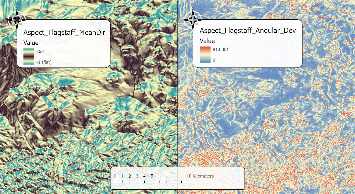
The output arrives symbolized for its statistic. Mean Direction and Median Direction get a cyclic aspect color scheme: bluegreen through yellow and brown and back through yellow to bluegreen, so that 0° and 360°, the same direction, share the same color, on a fixed 0° to 360° stretch, so that a given direction always maps to the same color whatever the spread of the data. Flat neighborhoods (−1) are drawn separately in a pale tan mask color rather than as part of the ramp, and NoData is transparent. The other statistics get a blue-to-red stretch. Every output carries its statistics and histogram, and its metadata records the input raster, the statistic, the neighborhood and the settings used.
A tour of the dialog
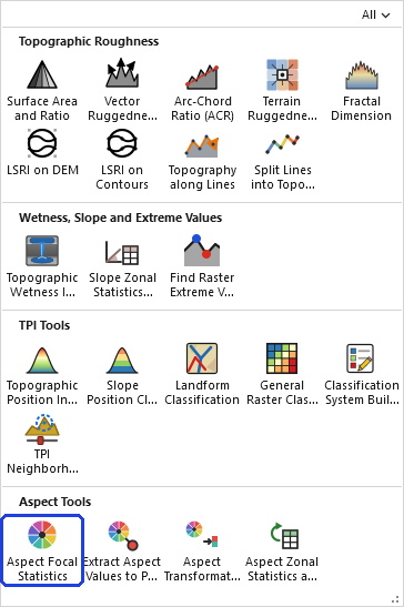
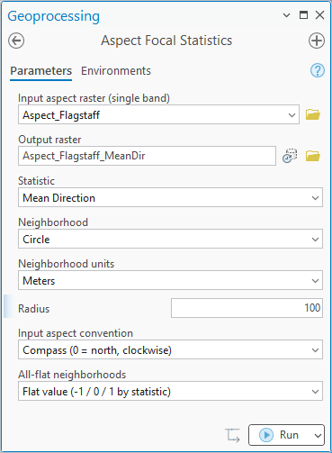
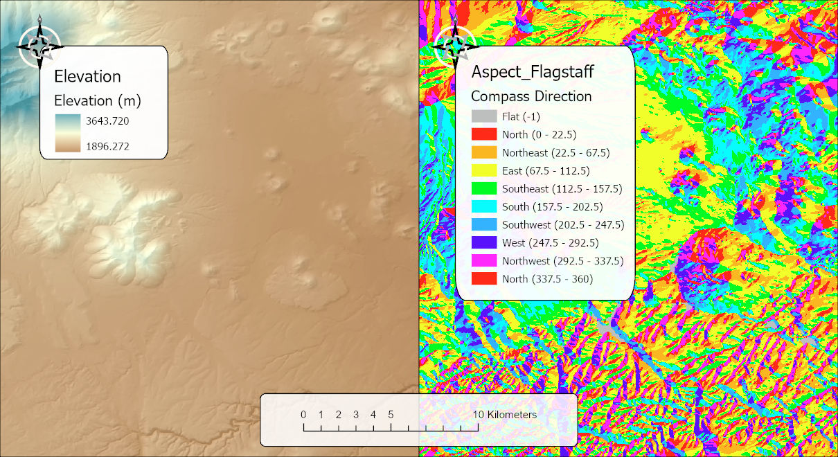
The dialog asks for the aspect raster, an output name, the statistic, the neighborhood shape and its size and units, the raster's direction convention, how to treat all-flat neighborhoods, and whether to ignore NoData. A name for the output is suggested from the input and the statistic.
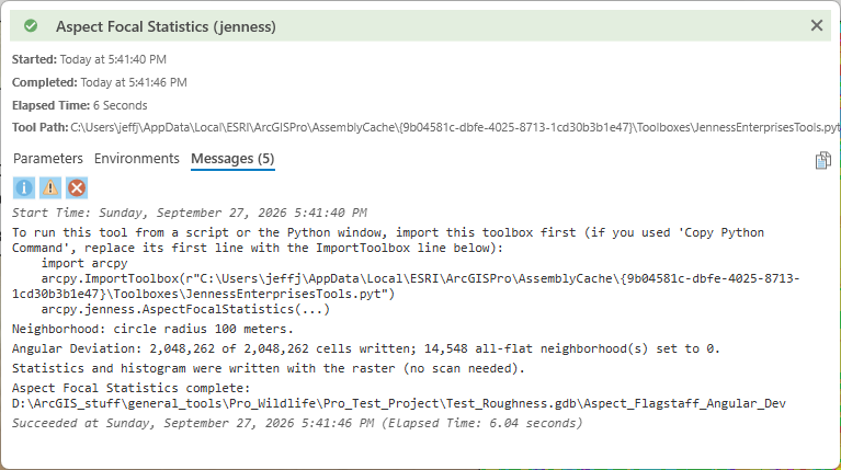
The tool holds the whole raster in memory at once, so the memory it needs grows with the number of cells. On most rasters that is no concern. On a very large one the tool may need more memory than your computer has free, and then one of two things happens: Windows starts using the disk as overflow memory and the tool slows to a crawl, or the tool stops with an out-of-memory error. There is no fixed limit; it depends on how much memory your computer has free. If a raster is too large, clip it to the area you need first.
ModelBuilder
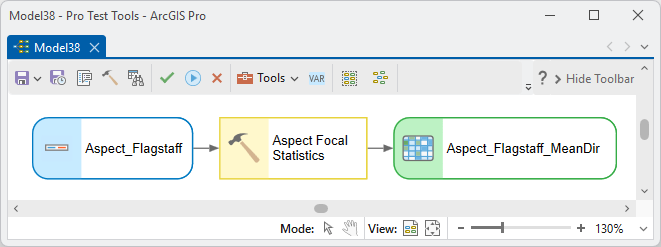
One run produces one statistic, so a model that needs, say, the mean direction and the circular variance runs the tool twice from the same input.
Parameters
| Label | Explanation | Data type |
|---|---|---|
| Input aspect raster (single band)Required · in_raster | A single-band aspect raster in degrees, 0–360 measured clockwise from north, with −1 for flat cells. A D-infinity flow-direction raster is also valid; set the convention to Mathematical for it. | Raster Layer |
| Output rasterRequired · out_raster | The output raster for the chosen statistic. A name is suggested from the input and the statistic. A folder path typed without an extension is written as a GeoTIFF. | Raster Dataset |
| StatisticRequired · statistic | The circular statistic to compute, one per run: Mean Direction, Median Direction, Mean Resultant Length, Circular Variance, Angular Variance, Circular Standard Deviation, Angular Deviation, Circular Range, Rayleigh Test p-value, von Mises Concentration (kappa), or Proportion With Defined Aspect. Default Mean Direction; the dialog remembers the last choice, as it does for the neighborhood shape, the neighborhood units, the all-flat option and the NoData option. | String |
| NeighborhoodRequired · neighborhood | Rectangle, Circle, Annulus, Wedge, Irregular or Weight. The size parameters below become active for the chosen shape. Default Circle. | String |
| Neighborhood unitsOptional · nbr_units | Cells, or a ground unit: Meters, Kilometers, Feet or Miles. On a geographic raster a ground unit is sized per row. Not used for kernel-file neighborhoods, which are defined in cells. Default Cells. | String |
| RadiusOptional · radius | The neighborhood radius for a Circle or Wedge, in the chosen units. Default 3. | Double |
| WidthOptional · width | The width of a Rectangle, in the chosen units. Default 3. | Double |
| HeightOptional · height | The height of a Rectangle, in the chosen units. Default 3. | Double |
| Inner radiusOptional · inner_radius | The inner radius of an Annulus, in the chosen units; cells inside it are excluded. Default 1. | Double |
| Outer radiusOptional · outer_radius | The outer radius of an Annulus, in the chosen units; must be greater than the inner radius. Default 3. | Double |
| Start angle (deg, CCW from east)Optional · start_angle | The starting angle of a Wedge, in degrees measured counter-clockwise from east. Default 0. | Double |
| End angle (deg, CCW from east)Optional · end_angle | The ending angle of a Wedge, in degrees measured counter-clockwise from east; the wedge spans counter-clockwise from the start angle to this one. Default 90. | Double |
| Kernel fileOptional · kernel_file | An ASCII text file for an Irregular or Weight neighborhood: the first line is “ncols nrows”, followed by the matrix, 0 and 1 for Irregular, weights for Weight. Centered on each cell, defined in cells. | File |
| Input aspect conventionRequired · input_convention | Compass (0 = north, clockwise) for ordinary aspect; Mathematical (0 = east, counter-clockwise) for a D-infinity flow-direction raster, whose Mean and Median Direction outputs are then converted to compass. Suggested automatically when a D-infinity raster is detected. | String |
| All-flat neighborhoodsRequired · flat_handling | What to write where every cell in a neighborhood is flat: Flat value, a per-statistic value from the table above, or NoData. Default Flat value. | String |
| Ignore NoData in calculationsOptional · ignore_nodata | Checked: NoData cells in a neighborhood are left out and the statistic uses the remaining cells. Unchecked: a cell is NoData when any cell of its neighborhood, or the area beyond the raster edge, is NoData. Default checked. | Boolean |
Python
The option strings are exactly as they appear in the dialog:
import arcpy
arcpy.ImportToolbox(r"C:\path\to\JennessEnterprisesTools.pyt")  # your install path

# ---- valid options for the list-driven parameters ------------------------
# statistic:         "Mean Direction", "Median Direction", "Mean Resultant Length",
#                    "Circular Variance", "Angular Variance",
#                    "Circular Standard Deviation", "Angular Deviation",
#                    "Circular Range", "Rayleigh Test p-value",
#                    "von Mises Concentration (kappa)",
#                    "Proportion With Defined Aspect"
# neighborhood:      "Rectangle", "Circle", "Annulus", "Wedge", "Irregular", "Weight"
# nbr_units:         "Cells", "Meters", "Kilometers", "Feet", "Miles"
# input_convention:  "Compass (0 = north, clockwise)",
#                    "Mathematical (0 = east, counter-clockwise; e.g. D-infinity)"
# flat_handling:     "Flat value (-1 / 0 / 1 by statistic)", "NoData"
# Unused neighborhood arguments may be left as they are; only the ones
# for the chosen shape are read.

# Circular mean aspect over a 3-cell-radius circle
arcpy.jenness.AspectFocalStatistics(
    in_raster=r"C:\Project\Terrain.gdb\aspect",
    out_raster=r"C:\Project\Terrain.gdb\aspect_MeanDir",
    statistic="Mean Direction",
    neighborhood="Circle", nbr_units="Cells", radius=3,
    input_convention="Compass (0 = north, clockwise)",
    flat_handling="Flat value (-1 / 0 / 1 by statistic)",
    ignore_nodata=True)

# Circular variance over a 5 x 5 rectangle
arcpy.jenness.AspectFocalStatistics(
    in_raster=r"C:\Project\Terrain.gdb\aspect",
    out_raster=r"C:\Project\Terrain.gdb\aspect_CVar",
    statistic="Circular Variance",
    neighborhood="Rectangle", nbr_units="Cells", width=5, height=5)

# A D-infinity flow-direction raster (mathematical convention); Mean
# Direction is converted to compass in the output.
arcpy.jenness.AspectFocalStatistics(
    in_raster=r"C:\Project\Terrain.gdb\flowdir_dinf",
    out_raster=r"C:\Project\Terrain.gdb\dinf_MeanDir",
    statistic="Mean Direction",
    neighborhood="Circle", nbr_units="Cells", radius=3,
    input_convention="Mathematical (0 = east, counter-clockwise; e.g. D-infinity)")
Recommended citation
Credits and references
By Jeff Jenness, Jenness Enterprises (www.jennessent.com). The tool is modeled on Esri's Focal Statistics; the circular statistics follow Mardia and Jupp (2000), Fisher (1993), Batschelet (1981) and Zar (1999), and the case for treating aspect as a direction is made in Jenness (2012).
- Batschelet, E. 1981. Circular Statistics in Biology. Academic Press, London. ISBN 0-12-081050-6.
- Best, D. J., and N. I. Fisher. 1981. The bias of the maximum likelihood estimators of the von Mises-Fisher concentration parameters. Communications in Statistics – Simulation and Computation 10:493–502. doi.org/10.1080/03610918108812225
- Esri. Focal Statistics (Spatial Analyst). ArcGIS Pro tool reference. pro.arcgis.com/en/pro-app/latest/tool-reference/spatial-analyst/focal-statistics.htm. Accessed on 27 September 2026.
- Fisher, N. I. 1993. Statistical Analysis of Circular Data. Cambridge University Press, Cambridge. doi.org/10.1017/CBO9780511564345
- Jenness, J. 2012. Issues with directional data. Remotely Wild, newsletter of the Spatial Ecology and Telemetry Working Group of The Wildlife Society. PDF
- Kish, L. 1992. Weighting for unequal Pi. Journal of Official Statistics 8:183–200. scb.se. Accessed on 29 September 2026.
- Mardia, K. V., and P. E. Jupp. 2000. Directional Statistics. Wiley, Chichester. doi.org/10.1002/9780470316979
- Zar, J. H. 1999. Biostatistical Analysis, 4th edition. Prentice Hall, Upper Saddle River, New Jersey. (Chapter 27, circular statistics; equation 27.4, the Rayleigh test p value.)
Licensing information
Works at every ArcGIS Pro license level (Basic, Standard, Advanced). No extension licenses are required; the neighborhood statistics are computed internally, without Spatial Analyst.
Related tools and pages
- About Aspect — why aspect matters, why it needs circular statistics, and how the Aspect Tools fit together.
- Extract Aspect Values to Points — aspect at point locations, interpolated as directions.
- Aspect Transformation — turns aspect into linear variables, such as northness and eastness, for use in ordinary statistics.
- Aspect Zonal Statistics as Table — the same circular statistics within zones rather than in a moving window.
- Projecting Rasters — project the DEM before computing aspect, not the aspect raster afterwards.