Spatially Balanced Sample (GRTS)

Geometric Tools · geoprocessing tool · by Jeff Jenness

Works at every ArcGIS Pro license level

Summary

Selects a spatially balanced probability sample from a point, polyline, or polygon frame using the generalized random-tessellation stratified (GRTS) design of Stevens and Olsen (2004) — the survey design behind many of the world's large environmental monitoring programs, as implemented in the spsurvey R package. Every location keeps its full, known inclusion probability, so design-based inference is exactly as sound as under pure random sampling — but each realized draw spreads over the frame the way pure randomness only promises on average.

The output is written in reverse hierarchical order, and that ordering is a practical field promise. Suppose you want to survey 30 sites and expect that a few will prove unreachable when you actually try — a landowner declines, a road washes out. Ask the tool for 30 base sites plus, say, 10 replacements, and plan on surveying the first 30 accessible sites in SiteID order: skip the locked gate, pick up the next site in the list. Because of the ordering, any leading run of SiteIDs — the first 10, the first 23, the first 30 — is itself a spatially balanced sample, and a run with a few skips filled from farther down the list remains very nearly so. Your final 30 stay balanced without redrawing anything. Each site also carries its design weight — in plain terms, how many hectares, line-meters, or frame units that site speaks for — so totals and means for the whole frame can be estimated without bias by simple weighted addition (the Horvitz-Thompson estimator, unpacked under Design weights and analysis).

“Frame” is a survey-sampling word, not a GIS word Throughout this page and the tool, the sampling frame is simply the geometry your sample is drawn from: the region within which sample sites are generated (polygons), the lines along which they are placed (polylines), or the set of candidate locations they are chosen from (points). GIS work rarely calls this a “frame” — words like study area, boundary, or analysis extent come to mind first — but the survey-sampling literature has long used sampling frame to mean the complete collection of everything that could possibly enter the sample, and Stevens and Olsen's papers and the spsurvey package both speak that language. We keep their word so this page reads side by side with the literature; just read “frame” as “the place, or the candidates, the sample comes from.”

This tool works on vector analysis areas — management area polygons, stream and trail polylines, or sets of points. It does not work on raster-based analysis areas. Esri offers a similar tool, Create Spatially Balanced Points, that does operate on raster datasets (but not vector datasets) using Dave Theobald's original algorithm (Theobald et al. 2007). Esri's tool requires the Advanced ArcGIS Pro license, or else the Geostatistical Analyst extension if you are licensed at the Basic or Standard ArcGIS Pro level.

The problem spatial balance solves

Start with what a simple random sample actually guarantees: nothing about your draw — only about the average over all possible draws. A perfectly legitimate random sample can put half its points in one corner of your study area and leave a quarter of it untouched. Both failures cost you, and in opposite ways: the clump wastes samples on closely spaced neighbors that echo one another (spatial autocorrelation — the same n_eff tax discussed on the Random Sample Array Generator page), while the void leaves part of the landscape's variety entirely unobserved. Ecological responses are almost always spatially structured, so a sample that covers the frame evenly nearly always estimates better — Stevens and Olsen's own simulations put GRTS variances at roughly half those of independent random sampling, and our implementation reproduces that figure.

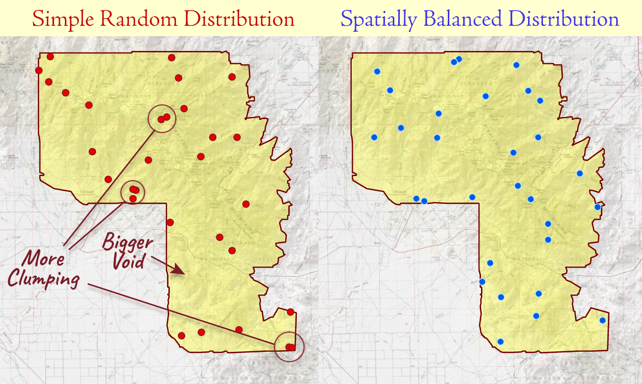
Two map panels of the same mountain-range boundary, 30 sample points in each: on the left, a simple random draw with three circled clumps of nearly touching points labeled More Clumping and a large empty region labeled Bigger Void; on the right, a spatially balanced draw from this tool with the same number of points spread evenly across the whole area — Thirty samples drawn by each approach over the same boundary. The simple random draw on the left is perfectly legitimate — and it still produced three tight clumps and left a substantial region unvisited. The spatially balanced draw on the right covers the same area with the same thirty points, no clumps, no void. Both are random samples; only one is *guaranteed* to look like this.

Is a balanced sample still a random sample?

It sounds like cheating — if the sample is guaranteed to spread out, hasn't some randomness been given up? Yes, in one precise sense; and no, in the sense that matters for inference. Split the worry into two questions. First: is any individual location now more or less likely to be sampled? No. Under GRTS, every location in the frame keeps exactly the same probability of being chosen as under pure random sampling — known, positive, and even-handed everywhere — and that is the entire foundation design-based inference stands on. Unbiased estimates, honest confidence intervals, inference to the whole frame: all of it survives untouched, because none of it ever required more. Second: can every combination of locations still occur together in one draw? No — and this is the only thing GRTS gives up. The draws that pile half the sample into one corner while ignoring the rest can no longer happen. Fewer possible samples exist, but every location is treated as fairly as ever. (In statistical language: the marginal inclusion probabilities are unchanged; only the joint distribution — which sites can co-occur — is restricted.)

And restricted randomization is not a suspicious novelty; careful restriction can increase the inferential power of the sample. Stratified sampling restricts randomness. Fisher's blocking restricts randomness. GRTS is literally stratification by random tessellation — invisible strata, nested all the way down, which is where the name comes from. The trade is entirely in your favor when the response is spatially structured: you give up sample configurations you never wanted (the clumped, voided ones) and keep the guarantee that made the sample defensible in the first place.

How the tool builds the sample

The construction is worth understanding, because every output field makes sense once you see it. Four steps:

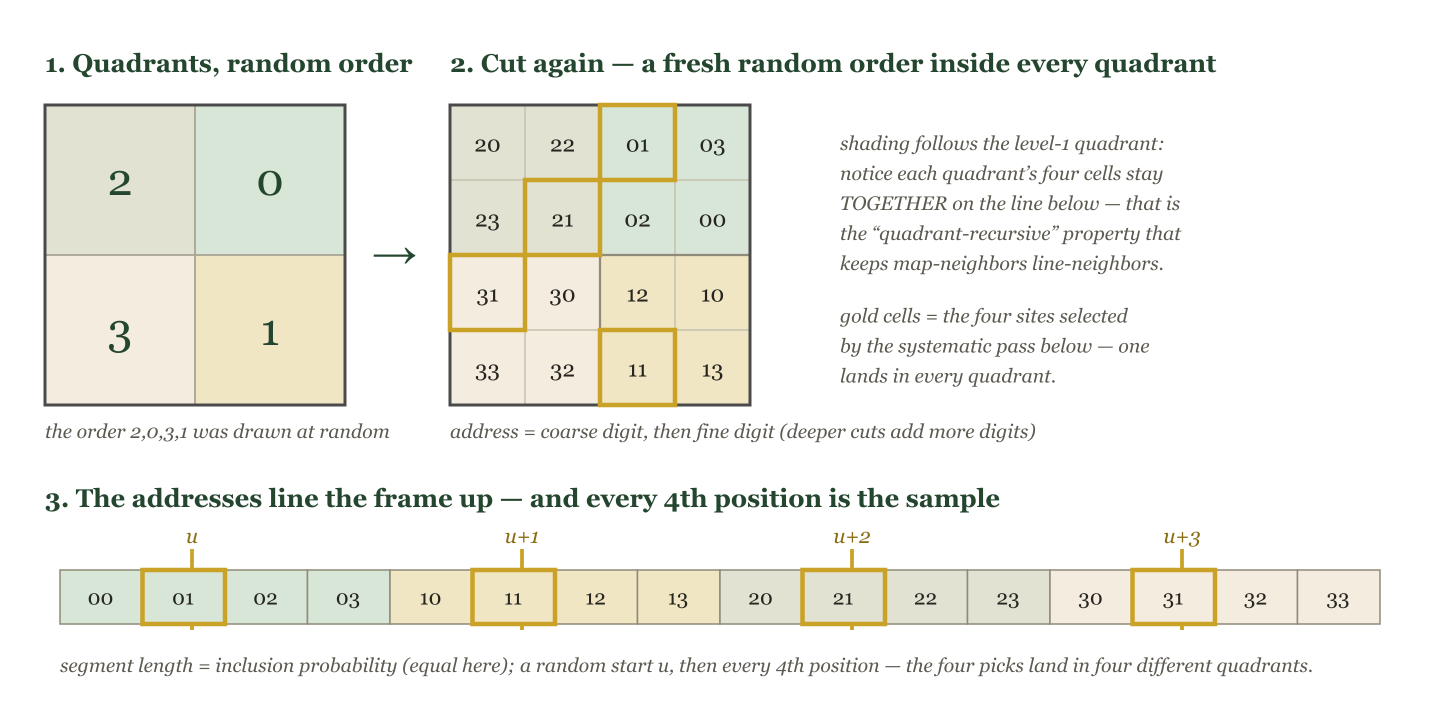
A randomly placed square, cut into quadrants, recursively. The frame is covered by a bounding square whose origin is shifted by a random offset (so no boundary between quadrants sits anywhere predictable). The square is cut into four quadrants, each quadrant into four sub-quadrants, and so on — and at every cut, the four pieces are put in a fresh random order. Reading the piece-labels from coarsest to finest gives every location a base-4 address, and because of the randomization, the addresses are unpredictable — yet locations near each other in space tend to share address prefixes, and that is the whole trick.
The frame becomes a line. Sorting by address lays the two-dimensional frame out along a one-dimensional line, with neighbors in space tending to stay neighbors on the line. Every sampling unit occupies a segment whose length is its inclusion probability — equal for an equal-probability design, proportional to the weight field for a probability-proportional-to-size (PPS) design, the length of line or share of area it represents for polyline and polygon frames.
One systematic pass selects the sites. A single random starting point u is drawn, and the sites at positions u, u+1, u+2, … along the line are selected. Systematic sampling on the spatially ordered line is what forces the selections apart in space — and because every segment's length equals its inclusion probability, each unit's chance of being hit is exactly what the design promised.
Reverse hierarchical ordering. Finally the selected sites are re-numbered by reversing the digits of their selection order (Stevens and Olsen's Table 1), which interleaves them so that the first 4 SiteIDs come from the four quarters of the design, the first 16 from the sixteen sixteenths, and so on: any leading run of SiteIDs is itself a spatially balanced sample. That single property is what makes ordered replacement sites possible.

Three-panel diagram: a square cut into quadrants labeled in the random order 2, 0, 3, 1; the same square cut again with a fresh random order inside every quadrant, giving each cell a two-digit address; and the sixteen addresses laid out as a line of segments, where a random start u and every fourth position select four sites that land one in each quadrant — The whole algorithm in one picture. Each level of cutting gets its own independently random order (panel 1's 2,0,3,1; panel 2's fresh shuffles inside each quadrant), and reading coarse digit then fine digit gives every cell an address. Sorting by address lays the frame out as the line in panel 3 — where each quadrant's cells stay *together* (the shading), which is the quadrant-recursive property that keeps map-neighbors close on the line. One random start u, one pick every 4th position — and the four gold picks land in four different quadrants of the map, spread out by construction. Deeper cuts add digits; unequal inclusion probabilities stretch or shrink the segments; everything else is bookkeeping.

Reading the output

The output is a point feature class whose order is part of the design:

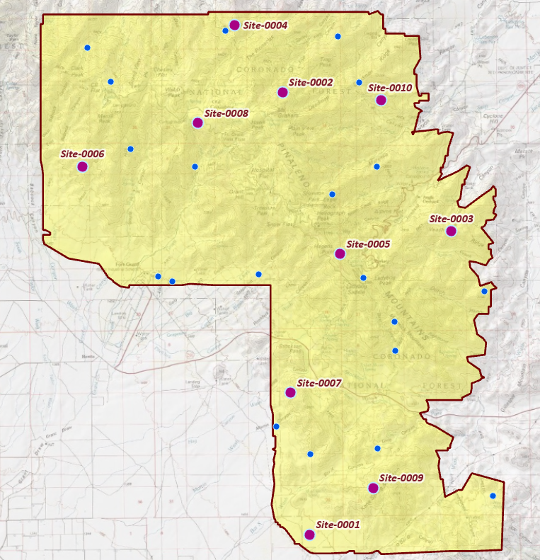
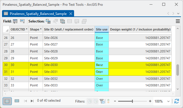
SiteID — the visit order. Site-0001 through Site-n are the base sample; visiting them in any order is fine, but if budget or survey conditions force you to visit only some of your samples, take that subset in SiteID order. For example, if you can only survey 10 of your samples then take the first 10 instead of a hand-picked 10, and you'll still have your spatially balanced sample.
Site_Use — Legacy (existing sites you required into the design), Base (the sample you intend to visit), or Over (the ordered replacement list).
Design_Wgt — 1 / inclusion probability: how much of the frame each site speaks for. These are the weights for Horvitz-Thompson estimation (below).
Stratum and Src_FID — when a stratum field was used, and (for point frames) the ObjectID of the source point.

A 30-site spatially balanced sample over the mountain-range boundary, with the first ten sites drawn larger in magenta and labeled Site-0001 through Site-0010, scattered evenly across the whole area; the remaining twenty sites are smaller blue dots filling in between them — The visit-order contract, visible. This is a 30-site base sample with the first ten SiteIDs highlighted — and notice that Site-0001 through Site-0010 already cover the whole block on their own, north to south, edge to edge. If the field season ended after those ten, you would still hold a spatially balanced sample; the remaining twenty (blue) fill in between them, refining the coverage rather than extending it. That is the reverse-hierarchical promise in one image.

An ArcGIS Pro attribute table showing rows Site-0026 through Site-0033 with columns for Site ID, Site use, and Design weight; the Site use column reads Base through Site-0030 and Over from Site-0031 on, with the two transition rows highlighted in yellow; every row carries the same design weight of about 14.2 million — The output table of a 30 + 10 design, caught at the seam: Site-0030 is the last Base site and Site-0031 the first replacement (highlighted rows). Nothing else changes at the boundary — the replacements are simply the design continuing past your requested 30. The design weight here is about 14,200,881 m² (roughly 1,420 ha) per site — the block's area divided evenly among the 30 base sites — and the replacements carry the same weight, so a substitute steps into exactly the share of the frame its unreachable predecessor spoke for.

Replacement sites: planning for locked gates

Field reality: landowners decline, roads wash out, a “lake” turns out to be a mudflat. Ask for replacement sites and the tool draws base + replacements as one spatially balanced design, then hands you the replacements at the tail of the SiteID order. When a base site cannot be visited, take the next unused Over site by SiteID — not the nearest one, not a judgment call — and the design stays as balanced as it can be. One honest caveat from Stevens and Olsen: the replacement pool is drawn inside the same design, so a huge reserve dilutes the base sample's balance a little — ask for a realistic number, not a bottomless one.

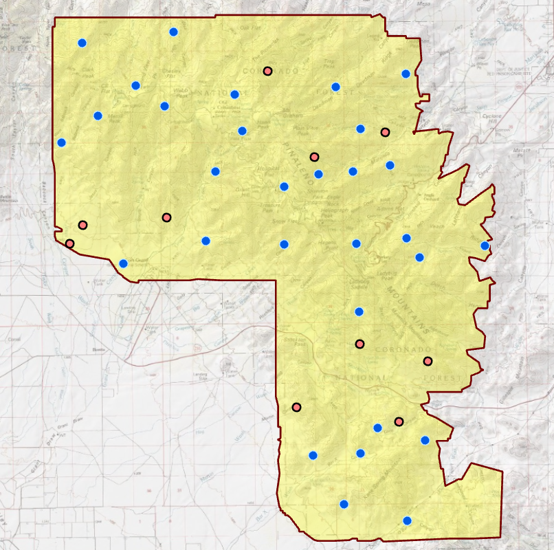
The mountain-range boundary with a 30 plus 10 design symbolized by Site use: thirty blue circle Base sites spread across the whole area, and ten red black-outlined Over replacement sites woven among them from the northern edge to the southern lobe — A 30 + 10 design symbolized by Site use: blue circles for the 30 Base sites, red symbols with black outlines for the 10 replacements. Notice that the replacements are woven through the same territory as the base sample — north, south, east, west — not huddled in a corner or stacked on the base sites. They were drawn in the same balanced design, so whichever one you reach for next is already positioned to patch the coverage a lost base site leaves behind.

One more piece of field planning: if you intend to hike to each site, the Estimated Shortest Path through Points tool will order your sites into an efficient field survey route — often a substantial saving in overall effort and time. Its help page's first figure is exactly this design, routed as a round trip from the truck.

Design weights and analysis

Every site carries its design weight, 1/π_i — the number of frame units (or hectares, or line-meters) it represents. The Horvitz-Thompson estimator, for all its imposing name, is nothing more than weighted addition: a site that represents 500 hectares contributes whatever you measured there, counted 500 hectares' worth, and a site representing 80 hectares counts 80 hectares' worth. After the field season, totals and means over the whole frame come from:

\hat{τ} = \sum_{i = 1}^{n} \frac{y_{i}}{π_{i}}

where y_i is whatever you measured at site i and π_i is its inclusion probability — an unbiased estimate of the frame total, for finite and continuous frames alike.

Variance is where a careful reader should slow down. The standard variance formulas in every statistics package — the machinery behind confidence intervals and significance tests — assume the sample was drawn by simple random sampling. Hand them a GRTS sample of a spatially structured response and they do not fail; they overstate. A balanced sample genuinely varies less from draw to draw than a random one of the same size (that is the entire point of balancing), and the formulas, knowing nothing of the balancing, report the larger simple-random figure anyway. Statisticians call that running conservative.

Why should you care? Because conservative errors are the safe kind, but they are not the free kind. Concretely: your confidence intervals come out wider than your data actually earned; a real trend or difference must be larger before your tests will declare it significant; and a monitoring program reporting to a funder looks less precise on paper than it truly is in the field. You paid the field costs for GRTS's extra precision — naive formulas simply decline to give you credit for it. Nothing is invalid: the intervals still cover at least their stated confidence, the tests still hold their error rates. When the uncredited precision matters, Stevens and Olsen (2003) built the local neighborhood variance estimator for exactly this situation, and the spsurvey R package implements it directly on this tool's output (the Design_Wgt field is the wgt column spsurvey expects).

One place you might meet this within our own suite: assessing a classification's accuracy with verification points drawn by this tool. The Classification Accuracy (Kappa) tools compute their kappa and overall-accuracy variances under the simple-random assumption, so with balanced points the estimates themselves — kappa, the accuracies, the error-adjusted areas — remain unbiased, while the reported confidence intervals run a little wide and the comparisons a little under-powered. Balanced verification points are still a fine choice (they see more of the map's variety than a purely random draw); just know the reports will be modest about the precision you actually achieved.

The balance report: putting a number on “spread out”

Every run reports how balanced the draw actually is, using the measure Stevens and Olsen themselves proposed. Start with the intuition you probably already have: draw the Voronoi cell of every base site — the region closer to that site than to any other — clip the cells to the frame, and in a perfectly balanced design of the ordinary equal-probability kind, all the cells should come out the same size. That intuition is exactly right, and for an equal-probability polygon frame the reported measure is precisely it. Each site “speaks for” the piece of the frame around it: call site i's share v_i, scaled so that a perfect design gives every site v_i = 1, and report the variance of the v_i as the imbalance.

The only reason the formal definition speaks of “inclusion probability” rather than “area” is the unequal-probability case. Picture the design's total inclusion probability — n units of it in all — spread across the frame before anything is drawn: uniform over an ordinary polygon frame, piled higher on heavily weighted units in a probability-proportional-to-size design. It is this spread-out, before-the-draw probability that each cell totals up — not the probability of the chosen site standing inside it (that would indeed always be a useless “100%”). A region carrying twice the probability was promised twice the sites, so a fair draw should cut it into twice as many cells; totaling probability rather than raw area keeps the measure honest in that case, and in the ordinary uniform case the two are exactly the same thing. (For a point frame, each cell simply totals the inclusion probabilities of the frame points inside it.)

The report also prints the Pielou evenness loss used by spsurvey (0 = perfect balance). For context: simple random samples typically score 2-3 times worse on both. And there is a satisfying way to see this number: run the Voronoi (Thiessen) Polygons tool on your design sites, clipped to the frame — roughly equal cells are spatial balance made visible.

The tool's run messages in ArcGIS Pro, highlighted: a 30 base plus 10 replacement areal design over a 426 million square meter frame, spatial balance Var(v) 0.158 and Pielou loss 0.0235 with the note that 0 is perfectly balanced and simple random samples typically run 2 to 3 times higher, the reverse-hierarchical-order explanation, and the line Random seed 42: this design is exactly reproducible — The report from a 30 + 10 run on the Pinaleños block (highlighted): the counts and frame size, the balance line — Var(v) 0.158, Pielou loss 0.0235, with the reminder that simple random samples typically run 2–3 times higher — the reverse-hierarchical-order promise spelled out, and the seed line that makes the whole design exactly reproducible. The two balance numbers are also handed to ModelBuilder as derived outputs.

The 40 spatially balanced design sites with their Voronoi cells clipped to the boundary, forming a honeycomb of similar-sized polygons, alongside the attribute table, a compact bell-shaped histogram of cell areas, and chart statistics highlighting a standard deviation of 324 hectares, minimum 438, maximum 1,922 — Balance made visible: 40 design sites created by **this Spatially Balanced Sample (GRTS) tool** (base and replacements together), run through our Voronoi (Thiessen) Polygons tool, with the area histogram and statistics alongside. The cells average 1,065.6 geodesic hectares, and they hold close to it: standard deviation 324 ha, the smallest cell 438 ha, the largest 1,922 ha, and a compact, bell-shaped histogram. Every site speaks for roughly its fair share of the block.

Forty simple random points through the same Voronoi treatment: cells of wildly varying size including tiny slivers in the southern clumps, a sprawling flat histogram, and chart statistics highlighting a standard deviation of 657 hectares, minimum 69, maximum 2,671 — The same treatment for 40 *simple random* points over the same block, created by the Random Point Generator tool. The mean is necessarily identical — the same total area divided among the same 40 cells — but look at the highlighted statistics: the standard deviation doubles to 657 ha, the smallest cell collapses to 69 ha (a sliver inside a clump of nearly touching points), the largest stretches to 2,671 ha (a cell left to cover a void alone), and the histogram sprawls where the balanced one bunched. Equal means, very different spreads — this is exactly what the report's Var(v) puts a single number on.

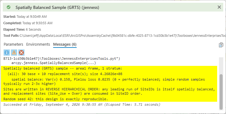
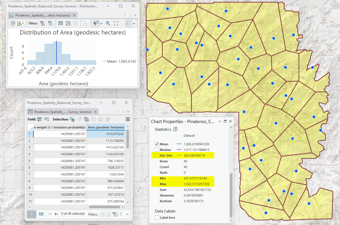
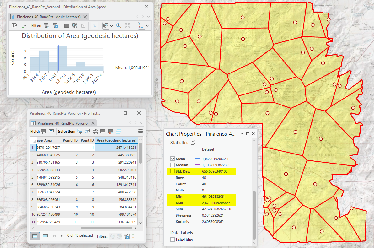
Both numbers are also returned as derived outputs (whole-sample Var(v) and Pielou loss), so a model or script can collect them without parsing the messages — see ModelBuilder below.

How we checked our work against R

The R package spsurvey (Dumelle and colleagues, including Olsen himself) is the reference implementation of the GRTS design — the code reviewers ask about when you write “we drew a GRTS sample” in a methods section. So before trusting this tool we put the two head to head: 100 independent designs of 50 sites each from the same mountain-range polygon, drawn by this tool, and another 100 drawn by spsurvey. Every one of the 200 samples was then scored with a single common yardstick — the same Var(v) calculation over the same fixed set of test points — so that neither implementation could grade its own homework.

The two distributions landed in the same place: our designs averaged Var(v) = 0.121, spsurvey's 0.138, and simple random samples of the same size scored 0.331 on the identical yardstick — both implementations beating pure randomness by the same comfortable factor of roughly 2.5 to 3. The small remaining gap has a known and rather satisfying explanation. spsurvey handles a polygon frame by approximating it with a finite cloud of candidate points (its pt_density argument controls how many), while this tool samples the polygon's continuous area exactly. Raise spsurvey's density and its balance walks steadily toward ours: 0.138 at the default density, 0.131 at ten times that, 0.128 at a hundred times — converging on our 0.121 as the approximation sharpens. In other words: the two implementations agree on the design, and this tool's continuous placement is the limit spsurvey approaches as its frame approximation densifies. Here is the full progression, every row a distribution of 100 independent 50-site designs scored on the identical yardstick:

Sample source	Frame representation	Mean Var(v)	Mean Pielou loss
spsurvey, `pt_density = 10` (the default)	500 random candidate points	0.1377	0.0175
spsurvey, `pt_density = 100`	5,000 candidate points	0.1313	0.0170
spsurvey, `pt_density = 1000`	50,000 candidate points	0.1280	0.0165
Spatially Balanced Sample (GRTS) — this tool	the continuous polygon, exact	0.1211	0.0156
Simple random sample (for context)	—	0.3308	0.0396

Reading the table statistically: each mean summarizes 100 independent designs whose draw-to-draw scatter gives it a standard error of about 0.003, so the gulf between the balanced designs and simple random (0.21 — some seventy standard errors) and this tool's difference from spsurvey's default (0.017 — about four) are far beyond chance. The individual steps of the middle rungs are smaller than that, and we do not lean on any one of them; what carries the evidence is that all four rungs land in the exact monotone order the convergence argument predicts in advance, with the distributions drawing measurably closer at every step.

Our conclusion, stated plainly: the tool has been validated head-to-head against the spsurvey package on identical frames. The two produce statistically equivalent designs, and the residual difference favors the exact continuous placement used here. The comparison is not a one-time ceremony, either — it lives on as a permanent automated test in the add-in's test suite, re-run whenever the sampling engine changes, alongside unit tests that reproduce Stevens and Olsen's published reverse-hierarchical-ordering example exactly and confirm over thousands of repeated draws that every unit's inclusion probability comes out as designed.

A tour of the choices

The frame — again, simply the geometry the sample is drawn from (see the note under the Summary) — can be points (each point a sampling unit — lakes, patches, candidate stations; the tool samples which units), polylines (the tool places sites along the lines), or polygons (sites within the polygons; holes respected). A layer's selection is honored. Geographic (latitude–longitude) frames are handled in an automatic equal-area working projection — a particularly happy pairing, because equal-area treatment is precisely what areal inclusion probabilities require — and written back in the input coordinate system.

The Geometric Tools gallery open on the ribbon, with the Spatially Balanced Sample (GRTS) button, in the Random Samples row, outlined in blue — Where to find it: **Spatially Balanced Sample (GRTS)** is in the *Random Samples* row of the *Geometric Tools* gallery, in the Geometric Tools group of the *Wildlife and Forestry* tab.

Stratification: give a stratum field and each stratum is sampled independently — its own hierarchical randomization, its own balance — with the totals split proportionally to stratum area/length/count (exact largest-remainder apportionment) or equally.

Unequal probability (PPS), point frames: a weight field makes each unit's inclusion probability proportional to its value — sample big lakes at four times the rate of small ones by giving them weight 4. Units whose scaled probability reaches 1 become certainties, included outright and handled exactly; the Design_Wgt field reflects it all.

Legacy sites, point frames: existing monitoring sites that must stay in the new design. They are guaranteed selection, labeled Legacy, and counted inside the base sample size — ask for 50 base sites with 5 legacy sites and you get those 5 plus 45 new ones.

Minimum distance between base sites: spatial balance already discourages close pairs, but when a hard minimum matters (independent camera stations, disease sampling), the tool redraws the design up to the Advanced retry limit and keeps the best draw, reporting plainly if any close pairs remain.

The Spatially Balanced Sample (GRTS) geoprocessing pane filled in: sampling frame Pinalenos, 30 base sites, 10 replacement sites, stratum field left blank, random seed 42, and the output named Pinalenos_Spatially_Balanced_Survey — The whole design in one small dialog: the Pinaleños frame, 30 base sites, 10 replacements, seed 42 — this is the very run whose report, attribute table, and maps appear throughout this page, and with that seed you can reproduce it to the site. Everything else is optional: a frame, a count, and an output name are all a basic run requires.

ModelBuilder

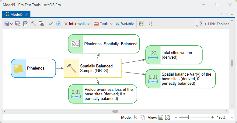
The tool offers a model the design-site feature class and three derived scalars: the total sites written, and the whole-sample spatial balance Var(v) and Pielou evenness loss from the balance report — so a model can, for instance, log the balance of every design it generates, or branch on it. The sample size chains in naturally from Estimate Sample Size's recommended count, exactly as with the Random Point Generator:

Parameters

Label	Explanation	Data type
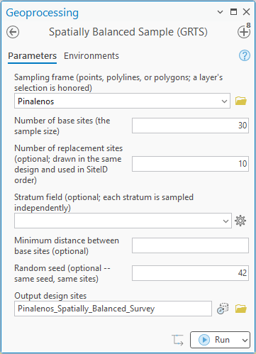
Sampling frameRequired · in_frame	Points (each a sampling unit), polylines (sites placed along the lines), or polygons (sites placed within; holes respected). A layer's selection is honored.	Feature Layer
Number of base sitesRequired · n_base	The sample size — the design you intend to visit. Legacy sites count toward this number.	Long
Number of replacement sitesOptional · n_over	Extra sites (Site_Use = Over) drawn in the same design, used in SiteID order when base sites prove inaccessible. A realistic reserve preserves balance better than a bottomless one.	Long
Stratum fieldOptional · stratum_field	An integer or text field defining strata; each stratum receives its own independent balanced sample.	Field
Allocation of sites across the strataOptional · alloc_method	Proportional to stratum size (area, length, or unit count; exact largest-remainder apportionment) or an equal count in each stratum.	String
Unequal probability (PPS) weight fieldOptional · aux_field	Point frames only: a non-negative numeric field; each unit's inclusion probability becomes proportional to it. Certainty units (probability 1) are handled exactly.	Field
Legacy sitesOptional · legacy_sites	Point frames only: existing sites (coinciding with frame points) guaranteed into the sample, labeled Legacy, counted inside the base size.	Feature Layer
Minimum distance between base sitesOptional · min_spacing	Honored by redrawing the design (best draw kept; plain warning if it cannot be fully met).	Double
Units for the minimum distanceOptional · linear_units	Meters, Kilometers, Feet or Miles.	String
Selection retriesOptional · max_tries	Advanced: how many fresh designs to draw in search of one meeting the minimum distance (default 10).	Long
Random seedOptional · random_seed	The same seed with the same inputs reproduces the same design exactly — cite it in a methods section.	Long
Output design sitesRequired · out_fc	The design sites in reverse hierarchical order: SiteID, Site_Use, Stratum, Design_Wgt, and Src_FID for point frames.	Feature Class
Total sites writtenDerived · out_n	Base + replacements, for ModelBuilder chains.	Long
Spatial balance Var(v)Derived · out_var_v	The whole-sample Voronoi balance of the base sites (0 = perfectly balanced; simple random typically 2-3× higher), for ModelBuilder and scripts.	Double
Pielou evenness lossDerived · out_pielou	The companion balance measure on a 0–1 scale (0 = perfectly balanced), for ModelBuilder and scripts.	Double

Python

A 50-site design over lake polygons with 10 ordered replacement sites, reproducible with a seed:

import arcpy
arcpy.ImportToolbox(r"C:\path\to\JennessEnterprisesTools.pyt")  # your install path
# alloc_method options (matching is by prefix):
#   "Proportional to stratum size (area, length, or unit count)"
#   "Equal count in each stratum"
# linear_units: "Meters" / "Kilometers" / "Feet" / "Miles"
result = arcpy.jenness.SpatiallyBalancedSample(
    in_frame=r"D:\data\study.gdb\lakes",
    n_base=50, n_over=10,
    random_seed=42,
    out_fc=r"D:\data\study.gdb\lakes_GRTS")
print(result.getOutput(1))  # total sites written
print(result.getOutput(2))  # spatial balance Var(v), 0 = perfect
print(result.getOutput(3))  # Pielou evenness loss, 0 = perfect

Recommended citation

Jenness, J. 2026. Spatially Balanced Sample (GRTS). Wildlife and Forestry Tools add-in for ArcGIS Pro, v. 1.82 (September 2026). Jenness Enterprises. Available at: https://github.com/JeffJenness/Wildlife_Tools.

Credits and references

By Jeff Jenness, Jenness Enterprises (www.jennessent.com). The generalized random-tessellation stratified design of Stevens and Olsen (2004), implemented as in the spsurvey package (Dumelle et al. 2023); spatial-balance metrics after Stevens and Olsen (2003); the GIS lineage of spatially balanced survey design after Theobald et al. (2007).

Dumelle, M., T. Kincaid, A. R. Olsen, and M. Weber. 2023. spsurvey: spatial sampling design and analysis in R. Journal of Statistical Software 105(3):1–29. doi.org/10.18637/jss.v105.i03
Robertson, B. L., J. A. Brown, T. McDonald, and P. Jaksons. 2013. BAS: balanced acceptance sampling of natural resources. Biometrics 69:776–784. doi.org/10.1111/biom.12059
Stevens, D. L., Jr., and A. R. Olsen. 2003. Variance estimation for spatially balanced samples of environmental resources. Environmetrics 14:593–610. doi.org/10.1002/env.606
Stevens, D. L., Jr., and A. R. Olsen. 2004. Spatially balanced sampling of natural resources. Journal of the American Statistical Association 99:262–278. doi.org/10.1198/016214504000000250
Theobald, D. M., D. L. Stevens Jr., D. White, N. S. Urquhart, A. R. Olsen, and J. B. Norman. 2007. Using GIS to generate spatially balanced random survey designs for natural resource applications. Environmental Management 40:134–146. doi.org/10.1007/s00267-005-0199-x

Licensing information

Works at every ArcGIS Pro license level (Basic, Standard, Advanced). No extension licenses are required — unlike Esri's Create Spatially Balanced Points, which requires an Advanced license or, at Basic or Standard, the Geostatistical Analyst extension.

Random Point Generator — unrestricted random designs with spacing and boundary-distance constraints; also the natural “pure random” comparison panel.
Random Sample Array Generator — whole sampling arrays per plot, and the autocorrelation discussion this page leans on.
Estimate Sample Size — how many sites the design needs; its derived count feeds this tool in ModelBuilder.
Voronoi (Thiessen) Polygons — draw the design sites' cells to see the balance the report scores.
Repeating Shapes — fully systematic designs, the opposite end of the randomness-regularity spectrum.
Select Random Records — aspatial random selection from existing records.
Estimated Shortest Path through Points — order the design sites into an efficient field survey route for hiking to every one.