

Find Raster Extreme Values
Summary
Finds the places where a raster surface reaches a local extreme and writes each one as a point. On a DEM those are the summits and the sinks. But nothing in the method assumes the surface is terrain, because the tool only ever compares one cell's value with its neighbors', so this tool finds local extremes equally well on any type of raster: run it on a slope raster and the “peaks” are the steepest points on the landscape and the “low points” the flattest; run it on a habitat-suitability surface and it finds the exact locations of the best and the worst habitat, the cores of the strongest patches and the centers of the least suitable ground; temperature, wetness, cost, density and probability surfaces all behave the same way. Each point carries the cell's value, its coordinates, a prominence (how far the extreme stands out from its surroundings, in the raster's own units) and a flag for extremes that sit on the edge of the data, because extreme points on the edge of a raster might not be true extremes. A flat summit or a flat-bottomed basin yields one point, not a cloud of them, and a flat bench partway down a hillside yields none. The extremes and their prominence are computed internally, so no Spatial Analyst license is needed.
What counts as an extreme
The two kinds of extreme are exact mirror images of each other, which is what lets one definition serve both. A low point is a cell, or a connected group of cells of equal value, with no lower neighbor among the eight cells around it. Water arriving there has nowhere to go: it is what the hydrology literature calls a sink, the cell with no outflow direction in the eight-direction (D8) flow model of O'Callaghan and Mark (1984). A peak is exactly the same thing on the upside-down surface: a cell or flat with no higher neighbor, which on a DEM is a summit. The tool therefore runs one procedure twice, once to find the low points on the true surface and once again to find the low points in the inverted surface, and labels the results Peak and Low Point.
That is not the only definition of a peak one could use. An earlier idea for this tool defined a peak as any cell with a flow accumulation of zero, meaning no upslope cell drains into it. It turns out that this describes every cell that simply has nothing above it, which is entire ridgelines, divide crests and the upper edge of every slope, often a quarter of a raster, rather than the summits themselves. The local-extreme definition finds the summits.
Flats need special handling, because integer DEMs are full of tied values, and a mesa top or a flat-bottomed basin can be hundreds of connected cells of exactly the same elevation. Every one of those cells has no higher (or no lower) neighbor, and reporting each of them as a peak would bury the map in points. The tool groups each connected region of equal extreme cells and writes a single point for it, placed at the region cell nearest the region's centroid, so that an L-shaped flat does not end up with its point hanging in space off the flat. A flat is treated as an extreme only when every known cell around its rim lies strictly on the wrong side of it: all strictly higher for a low point, all strictly lower for a peak. A flat bench partway down a hillside, a group of equal cells whose rim leads downhill on one side, is not an extreme and is excluded, and so is a flat that merely continues into cells that drain, since an equal cell beyond the rim means the flat goes on to somewhere with a way out.
Here is a small example to illustrate the methods. The grid below is a plane that falls from 60 on the west edge to 30 on the east edge, 5 per column, with three things added to it: a single cell raised to 70 near the northwest corner, a single cell dug out to 30 in the southeast quarter, and a bench of three equal cells at 45 running east-west across the middle, which begins at the column where the plane itself reads 50 and ends where it reads 40.
| 1 | 2 | 3 | 4 | 5 | 6 | 7 | |
|---|---|---|---|---|---|---|---|
| 1 | 60 | 55 | 50 | 45 | 40 | 35 | 30 |
| 2 | 60 | 70 | 50 | 45 | 40 | 35 | 30 |
| 3 | 60 | 55 | 50 | 45 | 40 | 35 | 30 |
| 4 | 60 | 55 | 45 | 45 | 45 | 35 | 30 |
| 5 | 60 | 55 | 50 | 45 | 30 | 35 | 30 |
| 6 | 60 | 55 | 50 | 45 | 40 | 35 | 30 |
| 7 | 60 | 55 | 50 | 45 | 40 | 35 | 30 |
Run through the tool, this grid yields exactly three points. The 70 at row 2, column 2 is a peak: all eight of its neighbors (60, 55, 50, 60, 50, 60, 55 and 50) are lower. The 30 at row 5, column 5 is a low point: its eight neighbors (45, 45, 35, 45, 35, 45, 40 and 35) are all higher. The third point is the entire east edge. Those seven cells all read 30, they form one connected flat, every cell along the flat's rim (the column of 35s) is strictly higher, so the flat is a low point, and the tool writes one point for it at the cell nearest the flat's centroid, row 4, column 7, flagged as being on the edge of the data. (The peak is flagged too, for a reason explained below: its prominence is measured against the edge.) The interior bench of 45 values does not produce an extreme point. Its westernmost cell has no lower neighbor of its own, but the flat it belongs to continues east to a cell whose neighbors include a 40 and a 35, so the flat drains and is not an extreme. The column of 60 values on the west edge does not produce an extreme point because it is adjacent to the peak at row 2, column 2. Nothing else on the grid qualifies: every remaining cell has at least one lower neighbor and at least one higher one, because the plane keeps falling to the east.
Prominence and depth
Every point carries a Prominence value. The tool computes it by merging cells in order of elevation. For low points it starts from the lowest cell and works upward, treating everything outside the raster as lower than any cell. Each low point starts its own group. Whenever a cell joins two groups, the group whose low point is the higher of the two is finished, and that low point is measured to the elevation of the joining cell, which is the saddle between the two basins. For a low point the number is therefore the depth of its own basin below the saddle where it joins a deeper basin, or below the spill point where it drains off the raster: how much water it would take to overflow it. For a peak, the same procedure runs on the inverted surface, from the summits downward, and the number it produces is the summit's topographic prominence: the vertical drop from the summit down to the key saddle, the highest pass you must descend to before you can climb to higher ground. Prominence, not elevation, is what separates a summit in its own right from a bump on a larger mountain's shoulder: a subsidiary summit has a small prominence no matter how high it is, because the saddle between it and the main summit is only a little below it.
The grid below shows both numbers on the same sloping plane as before, this time with two summits: 70 at row 2, column 2, and 66 two cells to its east, joined by a saddle cell of 58.
| 1 | 2 | 3 | 4 | 5 | 6 | 7 | |
|---|---|---|---|---|---|---|---|
| 1 | 60 | 55 | 50 | 45 | 40 | 35 | 30 |
| 2 | 60 | 70 | 58 | 66 | 40 | 35 | 30 |
| 3 | 60 | 55 | 50 | 45 | 40 | 35 | 30 |
The 66 is a peak in its own right, since its eight neighbors (50, 45, 40, 58, 40, 50, 45 and 40) are all lower. To reach higher ground from it you must descend to the 58 saddle before climbing to the 70, so its prominence is 66 − 58 = 8. The 70 is the highest cell on the grid, so there is no higher ground for it to be measured against. The tool then measures it against the raster edge: its region grows downward until it reaches the edge of the data, here the western column at 60, giving a prominence of 10, and the point is flagged (EdgeOfData = 1) because that number is a lower bound. The summit rises at least 10 above everything the raster can see; what lies beyond the edge is unknown, and the true prominence can only be larger. Any extreme whose path to higher (or lower) ground leaves the raster, or runs into NoData, is treated the same way: its prominence is the drop its region has made by the time it reaches the outside, and it is flagged. When two extremes in one basin are exactly equal, one is measured to the saddle between them and the other carries the basin's full depth. One consequence is worth knowing: an extreme that lies on the edge of the raster itself, or beside a NoData cell, like the east-edge flat in the first example, has made no drop at all when it meets the outside, so its prominence is exactly 0, and any positive prominence threshold removes it.
The minimum prominence parameter uses these values to screen out noise. At the default of 0 every raw extreme is kept. A real DEM produces thousands of one-cell bumps and pits, and at a modest positive threshold, say 10 elevation units, they disappear while the genuine summits and basins remain. The number generalizes to surfaces that are not terrain in the same way the extremes do: it reports how far the value stands above or below its surroundings before the surface crosses back. On a habitat-suitability surface, a maximum with a high prominence is a strong, distinct patch of good habitat, while one with a low prominence is a bump on a plateau that was already good, and the threshold separates the two.
The edge-of-data flag
Every point records, in an EdgeOfData field, whether its prominence was measured against the edge of the data rather than against real terrain. The field is 1 when the extreme's region reached the raster edge or NoData before it met higher (or, for a low point, deeper) ground, so the Prominence value is a lower bound, and 0 when the region met a real extreme inside the data and the value is exact. An extreme lying on the edge itself, or next to a NoData cell, is the limiting case: it has neighbors the tool cannot see, its “summit” may simply be where a ridge leaves the map, and its prominence is 0. Rather than silently dropping any of these, the tool writes every one and lets you screen them out with a definition query on the field when you want only fully known extremes. Flagged points are common on any real DEM: the highest summit and the lowest basin are always flagged, since nothing inside the data rises above the one or drains the other, and so is every extreme near the edge whose region reaches it first. No point is ever dropped for being on the edge.
The dominance radius
The dominance radius is a second, cruder filter, and it does two things at once. It enforces a separation distance between the reported points, since no two peaks, or two low points, can both survive if each lies inside the other's circle (unless the two are exactly equal, in which case both are kept), and it drops the lesser of any two extremes closer together than the radius, which is typically a small bump or hollow sitting beside a bigger feature. Unlike the prominence filter it never measures how far a point stands above or below its surroundings; a point is kept or dropped only by whether something more extreme lies within reach. The neighborhood is a circle centered on each extreme: every cell whose center lies within the radius of the point's center, so a diagonal neighbor counts the same as a cardinal one at the same distance. The default radius of 1.5 cells takes in exactly the eight immediate neighbors, because the four diagonal ones sit about 1.41 cells away and so fall inside 1.5, while a radius of exactly 1 would reach only the four cardinal neighbors, a plus-shaped neighborhood of five cells. That is the same convention as the neighborhood tools on the Terrain Ruggedness Index and its companion pages. Either way, every extreme already dominates its immediate neighbors by definition, so at any radius below 2 every regional extreme is reported and the filter does nothing. A larger radius keeps a point only if it is the most extreme cell in its circle: a radius of 10 keeps a peak only if nothing higher lies within 10 cells of it in any direction, and a low point only if nothing lower does. It is a quick way to thin dense terrain to its dominant features, and it can be combined with the prominence filter, in which case a point must pass both. Of the two, prominence is usually the more meaningful, because it describes the feature itself rather than its distance from a bigger one.
Coordinate systems
The output feature class is created in the raster's coordinate system unless the Output Coordinates geoprocessing environment is set, in which case that environment is honored. Most tools in this suite deliberately ignore the geoprocessing environments; this one respects this one, by design, because a point feature class is exactly the kind of output people want delivered in their working coordinate system. The X and Y attribute fields always report each point's coordinates in the output feature class's actual coordinate system, so the fields can never disagree with the geometry. Points are placed at cell centers. Because the algorithm compares cell values and nothing else, projected and geographic (latitude/longitude) rasters are handled identically; there is no distance or area in the calculation to be distorted.
Fields and symbology
Every field name is ten characters or fewer, so the output can be a shapefile as easily as a geodatabase feature class, and each field is documented in the output's field-level metadata. Points are written with the most prominent first, peaks before low points.
| Field | Contents |
|---|---|
| Type | Peak or Low Point. The field carries coded-value definitions for the two values. |
| SrcRaster | The name of the source raster, so the points remain traceable to the surface they came from. |
| SrcPath | The workspace the source raster was read from, up to 1,024 characters in a geodatabase; a shapefile holds 254, and a longer path is cut short with a warning. |
| CellValue | The extreme cell's value, in the raster's own units, whatever the raster measures: elevation on a DEM, slope on a slope raster, a suitability score on a habitat model. |
| Prominence | For a peak, the drop to its key saddle; for a low point, its depth below its spill point. A lower bound when EdgeOfData is 1. Raster units. |
| EdgeOfData | 1 if the prominence was measured against the raster edge or NoData (a lower bound; 0 for an extreme lying on the edge itself), 0 if it was measured against real terrain. |
| X, Y | The point's coordinates in the output feature class's coordinate system. |
The output arrives in the map with a Unique Values symbology on the Type field, blue for peaks and red for low points, so the two kinds can be distinguished at a glance.
A tour of the dialog
The examples use the same DEM as the Topographic Wetness Index page: the country just north of Flagstaff, Arizona, with 28.08 m cells in NAD 1983 UTM Zone 12N, running from 1,767 to 3,845 m. The San Francisco Peaks stand in the middle of the map, Doney Park and its cinder cones lie on the gentler ground to the east, and the whole area is on the Coconino National Forest.
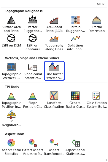
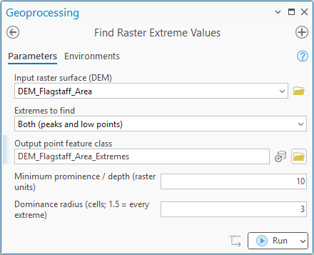
The dialog asks for the raster, which kind of extreme to find, an output name, and the two optional filters. With Both selected the peaks and low points go into a single feature class and the Type field tells them apart; the other two choices write only the one kind. Here the minimum prominence is 10 m, which removes the one-cell bumps and hollows that a 28 m DEM is full of, and the dominance radius of 3 drops any survivor that has a higher peak, or a lower low point, within three cells of it.
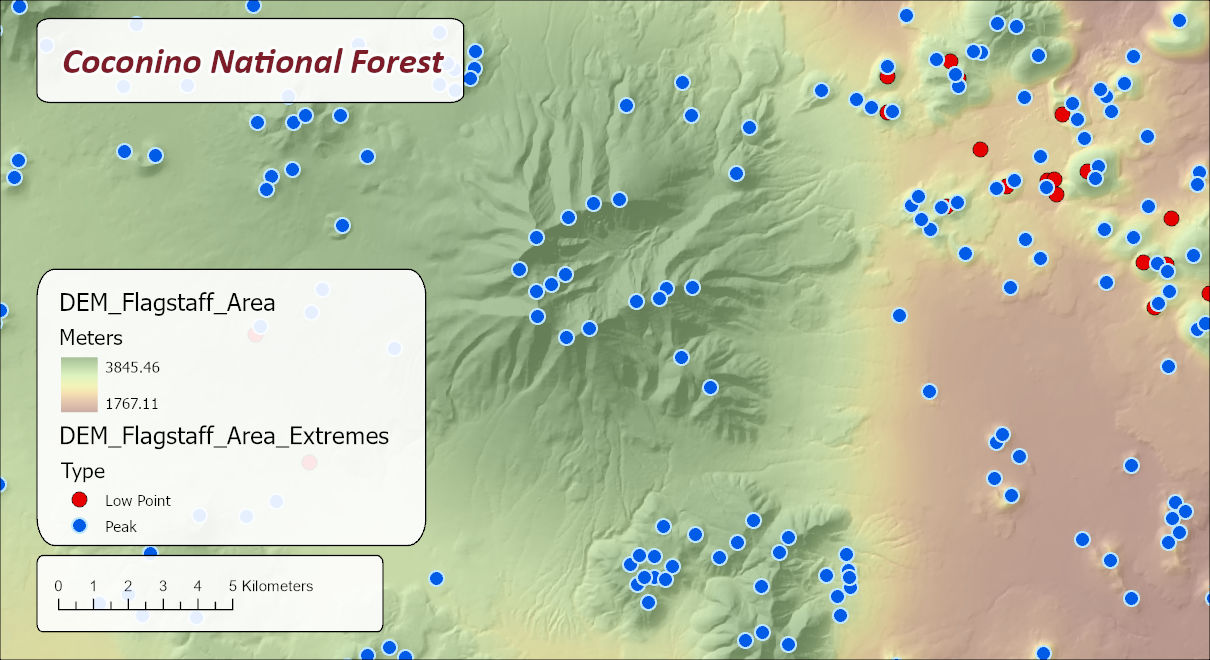
The map shows the two kinds of extreme sorting themselves by terrain. The peaks ring the summits and spur ends of the San Francisco Peaks and sit on top of the cinder cones to the east. The low points lie almost entirely in the cinder-cone country to the east, and many of them are not on low ground at all. The cinder hills of this area often have craters in their tops, and a crater bottom is a closed depression like any other: nothing drains out of it, so the tool marks it as a low point even though it sits well above the surrounding landscape. Several of the red points on the map are crater bottoms with a blue peak on the rim beside them. On the mountain itself nearly every hollow drains somewhere, so it is not a low point at all under the definition above, and the few closed depressions that exist there are shallower than the 10 m threshold. A low point, in other words, is a place water cannot leave, not a place that is low.
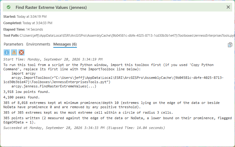
The run report shows how much work each filter did. The DEM holds 3,918 low points and 4,100 peaks, most of them the one-cell bumps and hollows of a 28 m surface, and the prominence threshold of 10 m removed all but 385 of them. The dominance radius removed none, because every extreme that survived the prominence filter was already the most extreme cell within 3 cells of itself; on this DEM the prominence threshold did all the thinning. The report also counts the points whose prominence was measured against the edge of the data, flagged EdgeOfData = 1: two here, neither of them anywhere near the edge of the map. One is the highest cell of the whole DEM, the summit of the San Francisco Peaks at 3,845 m. Nothing in the data stands higher, so the tool can only follow its slopes down until they connect with ground that reaches the raster boundary, which happens at 2,415 m, and report a prominence of at least 1,430 m. The other is a 3,169 m peak whose slopes reach the highest cell on the raster boundary, at 3,060 m, before meeting any higher ground inside the data. The highest summit of any DEM is always flagged this way, because no DEM contains the higher ground it would have to be measured against. Rerunning with a different threshold and comparing the maps is the quickest way to choose a prominence for a given DEM: raise it until the one-cell noise is gone and the features you recognize remain.
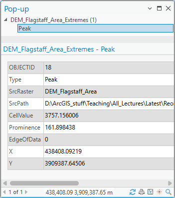
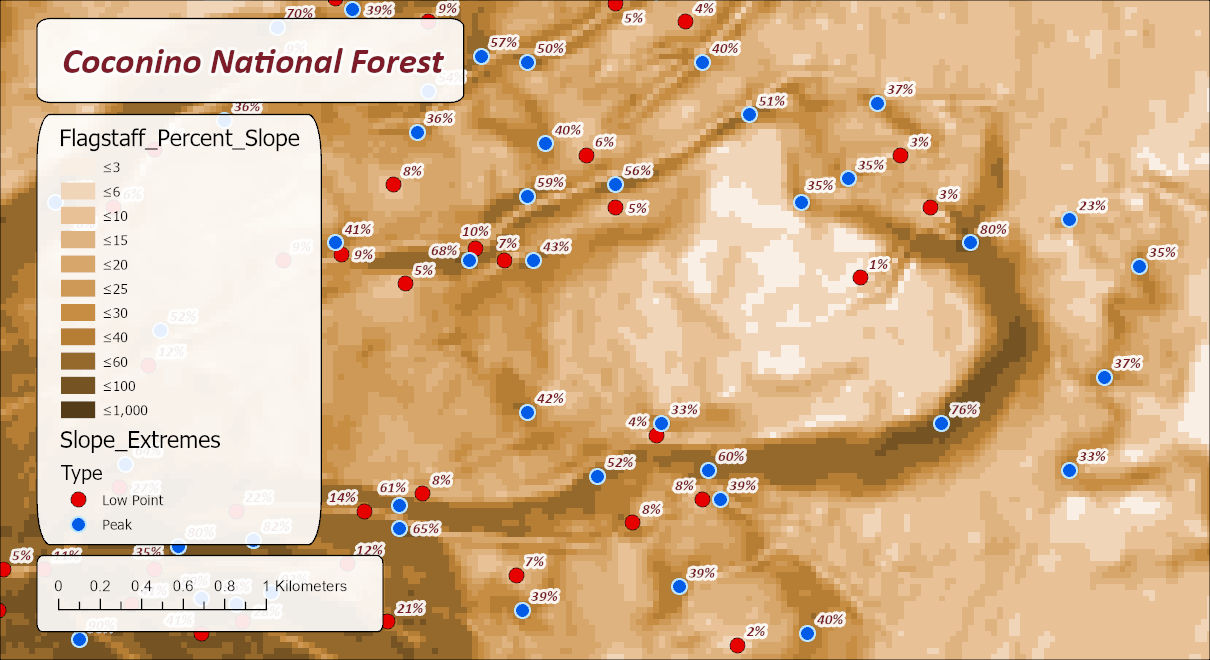
The slope run is the same tool with a different raster, and it answers a different question: not where the summits are, but where the ground is locally steepest and locally flattest. A blue point here is a cell with no steeper neighbor, a red one a cell with no flatter neighbor, and CellValue is the slope in percent rather than an elevation. Any continuous raster can be read this way.
The tool holds the whole raster in memory at once, so the memory it needs grows with the number of cells. On most rasters that is no concern. On a very large one the tool may need more memory than your computer has free, and then one of two things happens: Windows starts using the disk as overflow memory and the tool slows to a crawl, or the tool stops with an out-of-memory error. There is no fixed limit; it depends on how much memory your computer has free. If a raster is too large, clip it to the area you need first.
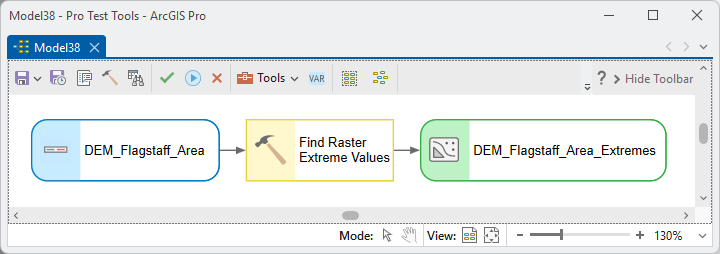
ModelBuilder
Parameters
| Label | Explanation | Data type |
|---|---|---|
| Input raster surface (DEM)Required · in_raster | The single-band raster whose extremes are to be found. A DEM gives summits and sinks, but any continuous surface works: a slope raster gives the steepest and flattest points, a habitat-suitability surface the best and worst habitat. NoData cells are ignored; an extreme beside them, or whose prominence is measured against them, is flagged in the EdgeOfData field. | Raster Layer |
| Extremes to findRequired · extreme_type | Both (peaks and low points), the default; Peaks (high points) only; or Low points only. With Both, the Type field distinguishes them in the single output. | String |
| Output point feature classRequired · out_fc | One point per extreme, in the raster's coordinate system unless the Output Coordinates environment overrides it. A name is suggested from the input. Fields: Type, SrcRaster, SrcPath, CellValue, Prominence, EdgeOfData, X and Y. | Feature Class |
| Minimum prominence / depth (raster units)Optional · min_prominence | Keep only extremes whose prominence (peaks) or depth (low points) is at least this many raster units. The default 0 keeps every raw extreme; a modest positive value removes the one-cell noise a real DEM produces. Any positive value also removes extremes lying on the edge of the data or beside NoData, whose prominence is 0. | Double |
| Dominance radius (cells; 1.5 = every extreme)Optional · window | Keep only extremes that are the most extreme cell within a circle of this radius, in cells, centered on them. The default 1.5 is the eight immediate neighbors, which every extreme already dominates, so it reports every regional extreme; 10 keeps a peak only if nothing higher lies within 10 cells of it in any direction. Combines with the minimum prominence. | Double |
Python
import arcpy
arcpy.ImportToolbox(r"C:\path\to\JennessEnterprisesTools.pyt")  # your install path
# Every peak and low point, with prominence / depth and the edge flag.
arcpy.jenness.FindRasterExtremeValues(
    in_raster=r"C:\Project\Elev.gdb\DEM",
    extreme_type="Both (peaks and low points)",
    out_fc=r"C:\Project\Elev.gdb\DEM_Extremes",
    min_prominence=0, window=1.5)
# Only the substantial features: prominence or depth of 20 units or more.
arcpy.jenness.FindRasterExtremeValues(
    in_raster=r"C:\Project\Elev.gdb\DEM",
    extreme_type="Both (peaks and low points)",
    out_fc=r"C:\Project\Elev.gdb\DEM_Big",
    min_prominence=20, window=1.5)
# Peaks only, delivered in the coordinate system set by the environment.
arcpy.env.outputCoordinateSystem = arcpy.SpatialReference(4326)
arcpy.jenness.FindRasterExtremeValues(
    in_raster=r"C:\Project\Elev.gdb\DEM",
    extreme_type="Peaks (high points) only",
    out_fc=r"C:\Project\Elev.gdb\DEM_Peaks",
    min_prominence=0, window=1.5)
arcpy.env.outputCoordinateSystem = None
# The third extreme_type string is "Low points only".
Recommended citation
Credits and references
By Jeff Jenness, Jenness Enterprises (www.jennessent.com). Prominence and depression depth follow the key-saddle definition, computed by merging cells in elevation order; the definition of a sink as a cell with no outflow direction follows O'Callaghan and Mark (1984).
- O'Callaghan, J. F., and D. M. Mark. 1984. The extraction of drainage networks from digital elevation data. Computer Vision, Graphics, and Image Processing 28:323–344. doi.org/10.1016/S0734-189X(84)80011-0
Licensing information
Works at every ArcGIS Pro license level (Basic, Standard, Advanced). No extension licenses are required; the extremes and their prominence are computed internally, without Spatial Analyst.
Related tools and pages
- Topographic Wetness Index — the toolbox's other tool built on sinks and flow, with its own depression fill and a choice of D8, MFD or D-Infinity routing.
- Slope Zonal Statistics as Table — summarize a slope raster by zone; this tool instead picks out the local extremes of any raster, a slope raster included.
- General Raster Classification — its worked example draws the peaks and low points from this page over a percent-slope raster.
- Topographic Position Index — where a cell stands relative to its neighborhood, rather than whether it is the extreme.
- About Topographic Roughness — the roughness measures, which describe terrain around a cell rather than picking out its extremes.
- Projecting Rasters — a DEM projected with nearest-neighbor resampling pools water “in places where no water would ever pool,” and every such place is a false low point; project DEMs bilinearly.