

MDOW Hillshade
Summary
Computes the Multi-Directional Oblique-Weighted (MDOW) hillshade of Mark (1992) from a single-band DEM. Four hillshades are made with the sun fanned out around a primary direction, and they are blended cell by cell with weights that depend on the aspect of the cell, so that every slope is lit mostly by the suns that strike it obliquely. Ridges and valleys that a single sun washes out because they run toward it come back into view. The tool is correct on latitude/longitude DEMs without projecting them, offers hypsometric shading and vertical exaggeration, and needs no Spatial Analyst license.
The idea
A hillshade with one sun has a blind spot. Any slope that faces the sun squarely is uniformly bright, any slope that faces straight away from it is uniformly dark, and in both cases the detail on the slope is lost; the hillshade only shows structure on the ground that the light rakes across at an angle. A ridge running toward the sun is drawn well, because the light crosses it; a ridge running across the sun is drawn as a bright wall and a dark wall with nothing on either. Moving the sun just moves the blind spot.
Robert Mark's answer (Mark 1992), devised to make a shaded-relief image of the Island of Hawaii, was to light the ground from four directions at once and, for each cell, to trust most the directions that light it obliquely. He computed four ordinary hillshades with the sun at 225°, 270°, 315° and 360°, all 30° above the horizon, and combined them with a weight for each that depends on the angle between the sun's direction and the aspect of the cell:
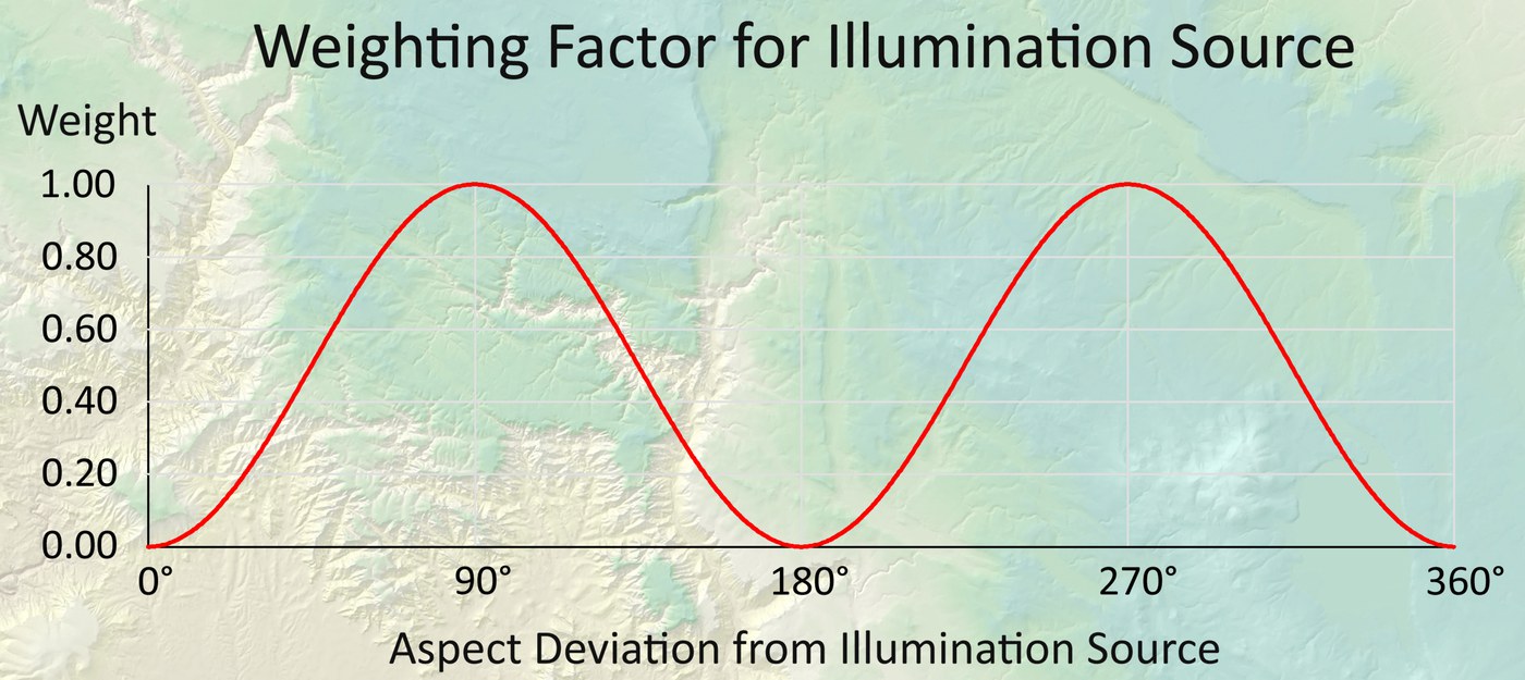
The weight is 0 when the cell faces directly toward the sun or directly away from it, and 1 when the sun is at right angles to the direction the cell faces, which is exactly the case in which a hillshade shows the most. The chart below is the weight for one sun as the aspect of the cell swings through the compass. (A slope facing away from a sun is dark in that sun's hillshade in any case; the weight simply says how much of that hillshade to use.)
Because the four directions are exactly 45° apart, the four weights for any cell always add up to exactly 2, so the blend is the weighted sum divided by 2:
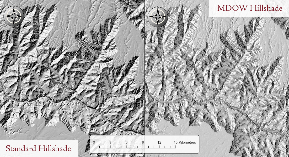
Every cell therefore ends up on the same scale as an ordinary hillshade, from 0 to one less than the number of gray levels. A flat cell, which has no aspect, gets the same value from all four suns and comes out at the brightness of flat ground under a sun 30° up. The lab exercise describes the effect as making the landscape look somehow glossy; whatever the word, structure appears in every orientation, and slopes that a single sun would have left as a flat gray or a flat black have their texture back.
How this tool applies the method
Mark fixed his four directions at 225, 270, 315 and 360 degrees because they suited Hawaii. This tool lets you set the Primary illumination direction, and fans the four suns around it at −67.5°, −22.5°, +22.5° and +67.5°. The default primary direction is 270°, following the legacy Surface Tools convention, which puts the suns at 202.5, 247.5, 292.5 and 337.5 degrees; Mark's own set is a primary direction of 292.5°, and the lab exercise uses 315°. All four suns share the one inclination, 30° by default as in Mark's report.
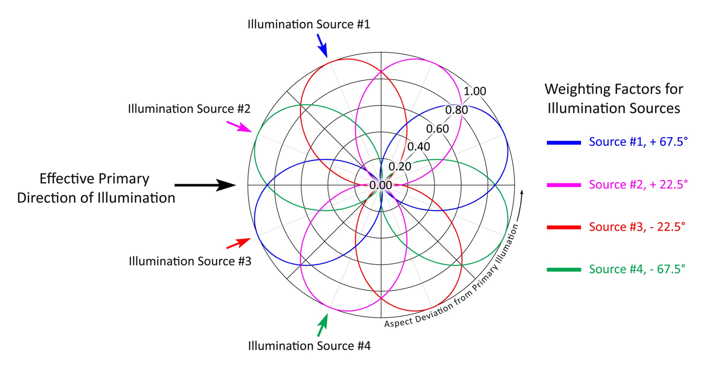
The chart below shows the weights of all four suns at once, drawn around the compass. The angle around the circle is the direction a cell faces, measured from the primary direction of illumination, and the distance from the center is the weight. Each sun's curve has two lobes at right angles to that sun's own direction, so whichever way a cell faces, the suns that light it most from the side carry the most weight.
Mark computed his weights from an aspect surface generalized to 1-kilometer cells, so that the weighting followed the broad grain of the island rather than every gully. This tool weights each cell by its own aspect, which gives a crisper result at full resolution. If you want something closer to Mark's smoother weighting, smooth the DEM first (Focal Statistics with a circular mean, as in the Blurred Hillshade recipe) and feed the smoothed DEM to this tool; the shading itself will then be generalized as well.
Each of the four hillshades is an ordinary one: ground that faces away from a sun gets no light from that sun, and its value is set to zero before the four are weighted and blended, as in Mark's method. (The legacy Surface Tools version, and early builds of this tool, blended the four first and set negative values to zero only at the end, which made slopes steeper than the suns' inclination, and turned away from one of the suns, darker than they should have been. This tool corrects that, so its result can differ from the legacy tool's on very steep ground.)
There is no cast-shadow option, as in the legacy tool: with four suns there is no single direction for a shadow to fall. The hypsometric-shading and vertical-exaggeration options work as they do in the Enhanced Hillshade, the hypsometric darkening being applied once, to the blended result. Geographic DEMs get the same per-row spheroidal cell dimensions as the other tools, so no projection is needed, and the elevation units are read from the DEM's vertical coordinate system when it has one.
A tour of the dialog
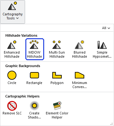
The tool opens from the Cartography group of the Wildlife and Forestry Tools ribbon tab or from the Cartography Tools toolset of the Jenness Enterprises toolbox.
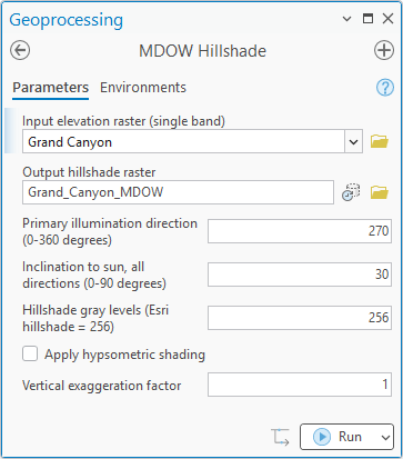
Choose the DEM and accept or change the suggested output name. The Elevation units row appears only when the tool cannot tell what the elevation units are; when the DEM declares its vertical units, or is in geographic coordinates, Pro hides the row, as in the pane above. The Primary illumination direction is the center of the fan; the tool's messages list the four sun directions it produces. The Inclination applies to all four suns. The number of Hillshade gray levels defaults to 256, which gives values from 0 to 255, the same range as Esri's hillshade; a small number gives a posterized result, and 32 or fewer adds a raster attribute table. Hypsometric shading and vertical exaggeration are optional and off by default. Your last choices are remembered with the project.
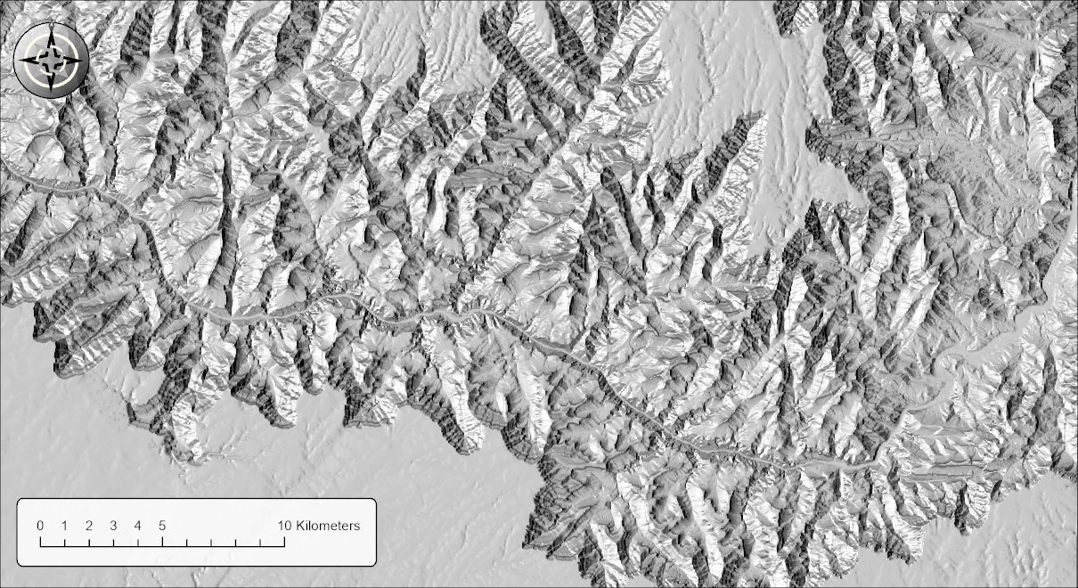
The output is a 16-bit integer raster from 0 to one less than the number of gray levels, NoData where the DEM is NoData and at its edge, with statistics, a histogram and bilinear pyramids already built, drawn on arrival with a black-to-white stretch whose white is the highest value present (or, at 32 or fewer gray levels, with unique values, one gray for each level). The whole computation runs in strips, so DEM size is not a concern.
Environment settings
By default the output matches the input DEM exactly. Processing Extent, Snap Raster, Cell Size and Output Coordinate System are honored as finishing steps applied to the computed hillshade, so the shading is always computed from the full-resolution DEM and then clipped, resampled or reprojected. The Mask environment is not honored, and pyramids are always built with bilinear resampling.
ModelBuilder
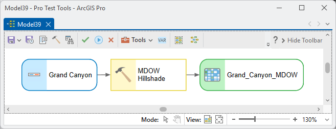
In a model the tool takes one input, the DEM, and produces one output, the MDOW hillshade raster. The four hillshades, the aspect surface and the weighting all happen inside the tool.
Parameters
| Label | Explanation | Data type |
|---|---|---|
| Input elevation raster (single band)Required · in_raster | The DEM. Must be single band; projected or geographic. Choose a layer from the map or browse to a dataset. | Raster Layer |
| Output hillshade rasterRequired · out_raster | The MDOW hillshade (integer, 0 to one less than the number of gray levels). NoData where the DEM is NoData and at its outer edge. A name is suggested from the input. | Raster Dataset |
| Elevation unitsOptional · elev_units | Meters or Feet. Read from the DEM's vertical coordinate system when it has one; geographic DEMs are assumed to be in meters. In both cases the row is hidden in the dialog; you are asked only when the DEM does not say. | String |
| Primary illumination direction (0-360 degrees)Required · azimuth | The center of the fan of four suns, which sit at −67.5, −22.5, +22.5 and +67.5 degrees from it. The default 270 (west) gives 202.5, 247.5, 292.5 and 337.5. | Double |
| Inclination to sun, all directions (0-90 degrees)Required · altitude | The height of all four suns above the horizon. The default 30 follows Mark (1992). | Double |
| Hillshade gray levels (Esri hillshade = 256)Required · levels | The number of gray levels; output values run from 0 to one less than this number. The default 256 matches Esri's 0 to 255; 32 or fewer adds a raster attribute table. | Long |
| Apply hypsometric shadingOptional · use_hypso | Darkens low elevations by the strength below, applied to the blended result. Off by default. | Boolean |
| Hypsometric strength (0-100)Optional · hypso_strength | At strength s, the brightness multiplier runs from (100 − s) percent at the lowest elevation to 100 percent at the highest. The default is 50. | Long |
| Vertical exaggeration factorOptional · vert_exag | Multiplies the elevations before shading. The default is 1. | Double |
Python
import arcpy
arcpy.ImportToolbox(r"C:\path\to\JennessEnterprisesTools.pyt")  # your install path
# Mark's own four directions (225, 270, 315, 360) are a primary direction of 292.5.
arcpy.jenness.MDOWHillshade(
    in_raster=r"C:\Project\Elev.gdb\DEM",
    out_raster=r"C:\Project\Elev.gdb\DEM_MDOW",
    elev_units="Meters", azimuth=292.5, altitude=30, levels=256,
    use_hypso=True, hypso_strength=40, vert_exag=1)
Recommended citation
Credits and references
By Jeff Jenness, Jenness Enterprises (www.jennessent.com), implementing the method of Mark (1992). A port of the MDOW function in the author's DEM Surface Tools for ArcGIS (Jenness 2013). The gradient is Horn's (1981).
- Horn, B. K. P. 1981. Hill shading and the reflectance map. Proceedings of the IEEE 69:14–47. doi.org/10.1109/PROC.1981.11918
- Jenness, J. 2013. DEM Surface Tools for ArcGIS (v. 2.1.375). Jenness Enterprises. jennessent.com/arcgis/surface_area.htm
- Jenness, J. Raster lab 12: Hillshades with Swiss Method effects in ArcGIS Pro; MDOW. Lab exercise video, GIS training courses, Jenness Enterprises. youtu.be/DP309q778Vw
- Mark, R. K. 1992. A multidirectional, oblique-weighted, shaded-relief image of the Island of Hawaii. U.S. Geological Survey Open-File Report 92-422. doi.org/10.3133/ofr92422
Licensing information
Works at every ArcGIS Pro license level (Basic, Standard, Advanced). No extension licenses are required; the four hillshades and their blending are computed internally, without Spatial Analyst.
Related tools and pages
- About Hillshades and the Swiss Method — the five tools compared.
- Multi-Sun Hillshade — the other multiple-light tool: suns you place, weights you set, no aspect weighting.
- Enhanced Hillshade — the single-sun tool, with cast shadows.
- Blurred Hillshade — the softening component.
- Simple Hypsometric Shading — drape an elevation tint over the MDOW result.
- About Aspect — the quantity the weights depend on.
- Projecting Rasters — this tool works on geographic DEMs directly; if you project a DEM first, use bilinear interpolation.