

Blurred Hillshade
Summary
Computes a deliberately softened hillshade from a single-band DEM: the blurring component of the Swiss method. You choose a radius, in cells or in ground units, and whether to blur the DEM before shading it (the default, which generalizes the terrain itself) or to blur the finished hillshade afterward (which softens every tonal edge, shadows included). The blur is a circular average or a Gaussian, sized per row on the spheroid for latitude/longitude DEMs. Every option of the Enhanced Hillshade is here as well: correct geographic handling, hillshade gray levels, hypsometric shading, vertical exaggeration and soft cast shadows. No Spatial Analyst license is needed.
The idea
Some people like to blur a hillshade so that it is visually softer and less distracting under the rest of the map. Kurt Brassel, who first automated the Swiss cartographers' hand-drawn relief conventions, gave a more principled reason (Brassel 1974): the smallest terrain features are described by the fewest data points, so their shading is the least trustworthy, tending, in his words, to be “fictive” or “creative,” and he argued that they should be blurred to de-emphasize them. He was also printing his hillshades on a line printer from the 1960's, and photographically blurring the output improved them a good deal. (For a simulated example of his line-printer output, before and after blurring, see the About Hillshades page.) The USGS uses a softened hillshade beneath its topographic maps, where a crisp one would fight with the contours. Buckley and Barnes (2004), in an Esri conference session on cartographic effects, recommend smoothing for the same reason, as the thing to do “if you really want the hillshade to recede into the background a bit more,” and they smooth both ways this tool offers: a neighborhood mean of the DEM before shading it, and a circular mean of the finished hillshade. Not everybody agrees that a blurred hillshade is more attractive, though, so give the result some careful thought before you adopt it.
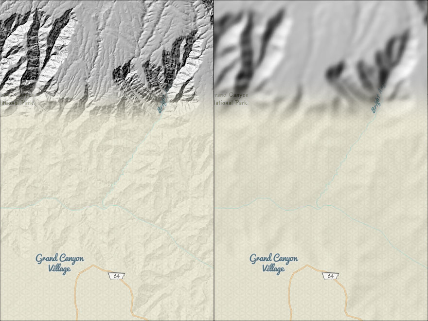
Two ways to blur
The What to blur parameter chooses between them, and they give different pictures.
DEM (blur before shading), the default and the lab's recipe, averages the elevations within the radius and computes the hillshade from that smoothed terrain. Small landforms are removed from the terrain itself, so they disappear from the picture, while the larger forms that remain are shaded crisply; cast shadows and hypsometric shading follow the generalized surface. In my experience, this option usually looks a little better, but then again beauty is in the eye of the beholder. This tool gives you a choice.
Hillshade (blur after shading) computes the normal hillshade first and then blurs the finished image, as Brassel blurred his prints. Every tonal edge softens, the sharp line of a cast shadow becomes a soft penumbra, and the result is closer to what an out-of-focus photograph of a relief model would give. The small landforms are still there; they are just drawn softly.
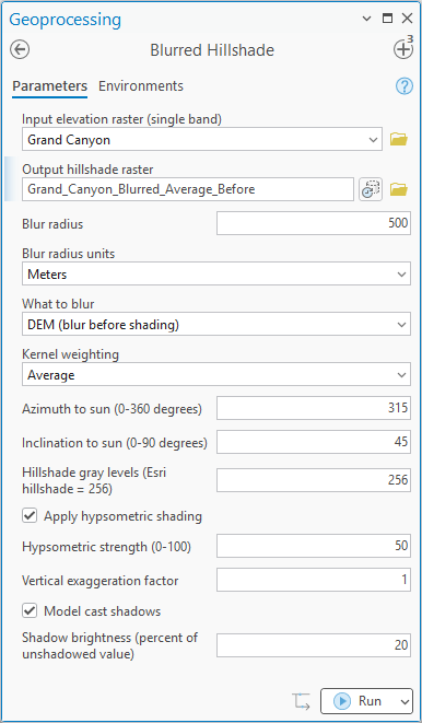
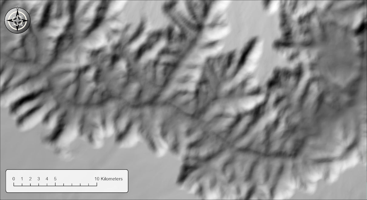
The two hillshades below come from the same DEM and the same settings, a Gaussian blur with a radius of 500 meters, and differ only in what was blurred.
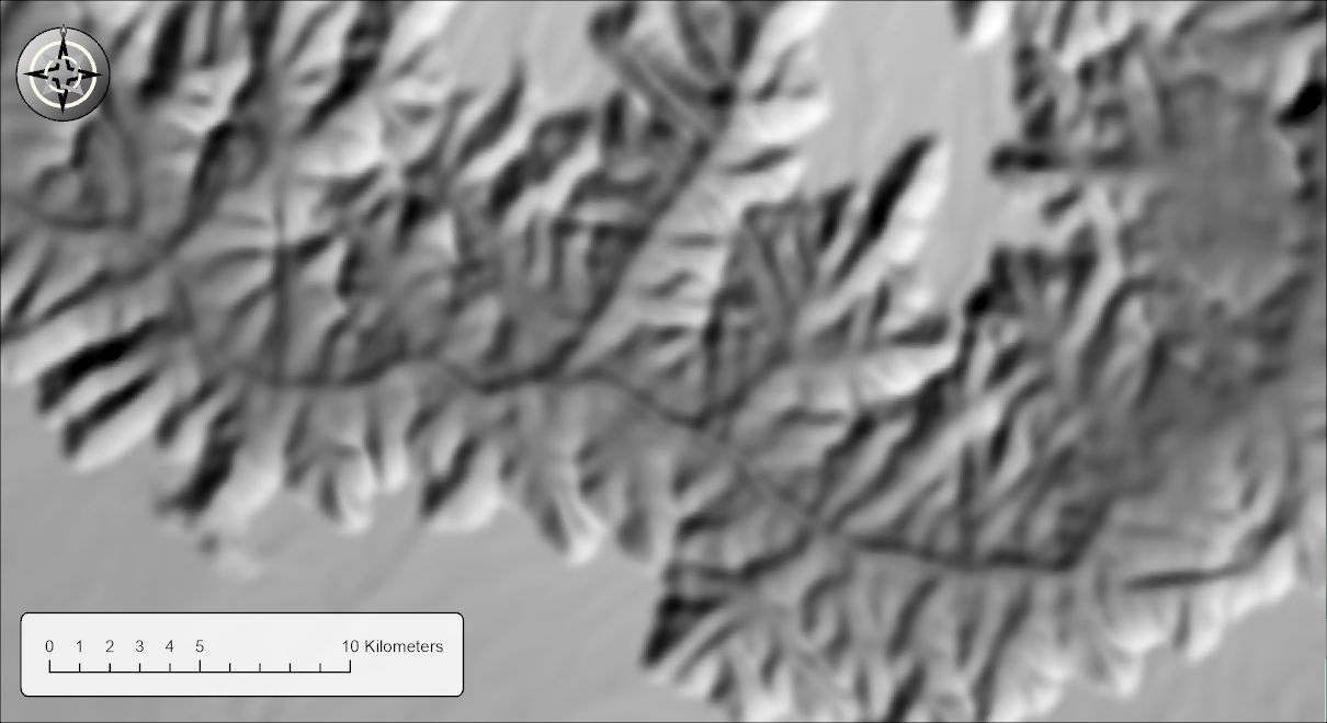
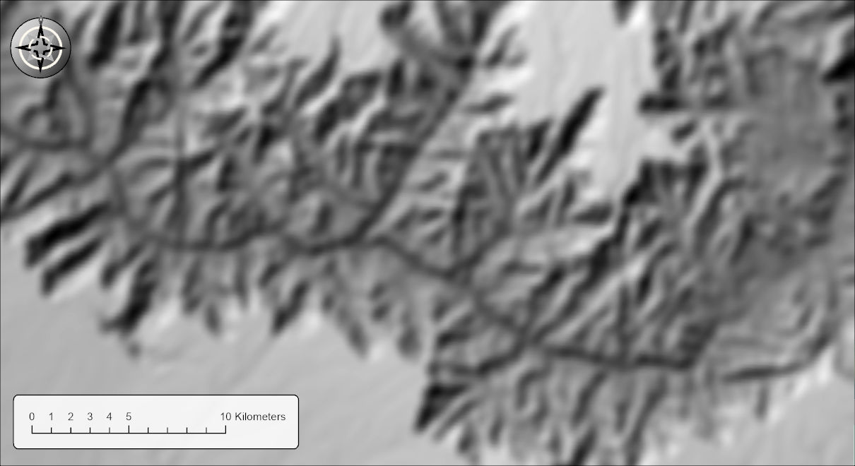
What is the difference to you? Blurring the DEM changes the terrain, and blurring the hillshade changes only the picture. With the DEM blurred first, the tool shades a simpler landscape: the side canyons and small ridges narrower than the blur are gone, and what remains is drawn in focus, as smooth, rounded forms with a clean boundary between their lit and shaded sides. With the hillshade blurred afterward, nothing has been removed from the terrain. The shading and the shadows are those of the full-detail DEM, but the whole picture has gone out of focus and the fine detail smears into its surroundings. Blur the DEM when you want a generalized terrain, in which only the main landforms matter. Blur the hillshade when you want the real terrain, just softened, so that it sits back behind the rest of the map.
The radius and the kernel
The blur is a circular mean: each cell is replaced by the average of the cells within the radius. The radius can be given in cells, which applies the same neighborhood everywhere, or in meters, kilometers, feet or miles, which the tool converts to cells from the cell size, planarly for a projected DEM and row by row on the spheroid for a geographic one, so that the circle stays the right size at every latitude. NoData cells are ignored and stay NoData; cells near an edge average whatever valid neighbors fall inside the circle. The right radius depends on the resolution of the DEM and on how far in your map is zoomed; the lab's advice is that you will almost certainly try several values before you settle on one you like. The default is 10 cells, the lab's value. A radius smaller than one cell reaches no neighboring cells and blurs nothing; the tool warns you when that happens.
The Kernel weighting decides how the cells inside the circle are weighted. Average weights them all equally, which is what Focal Statistics does and what the lab uses. It is the original method offered by the Jenness tools. Gaussian, added in this version, weights them by distance from the center, with a standard deviation of half the radius and nothing beyond the radius; the falloff is smoother, it avoids the faint box-like or ring-like artifacts a uniform average can leave around sharp features at larger radii, and the result looks a little smoother.
Blurring needs the whole DEM in memory at once, unlike an ordinary hillshade, which is computed in strips, and that matters on a very large DEM. A calculation done in strips uses about the same modest amount of memory however large the DEM is, while the blur uses memory in proportion to the number of cells, about 90 bytes per cell at its peak, whichever kernel and whichever What to blur option you choose. A DEM of 5,000 by 5,000 cells (25 million cells) therefore needs a little over 2 gigabytes, which most computers can spare. A DEM of 10,000 by 10,000 cells (100 million cells) needs about 9 gigabytes, and one of 20,000 by 20,000 cells about 36 gigabytes, which is more than many computers have free. Past what your computer can spare, one of two things happens: Windows starts using the disk as overflow memory and the tool slows to a crawl, or the tool stops with an out-of-memory error. There is no fixed limit, then; it depends on how much memory your computer has free. The blur itself is quick, a matter of seconds for tens of millions of cells. If a DEM is too large to blur, clip it to the area you need first.
Everything else
Beyond the blur, the tool offers the same options as the Enhanced Hillshade: one sun at an azimuth and inclination (315 and 45 by default), correct on geographic DEMs through per-row spheroidal cell dimensions, elevation units read from the DEM's vertical coordinate system, a chosen number of gray levels, hypsometric shading, vertical exaggeration, and cast shadows dimmed to a chosen brightness. With the DEM blurred first, the shadows are cast by the generalized terrain; with the hillshade blurred after, their edges are softened by the blur.
A tour of the dialog
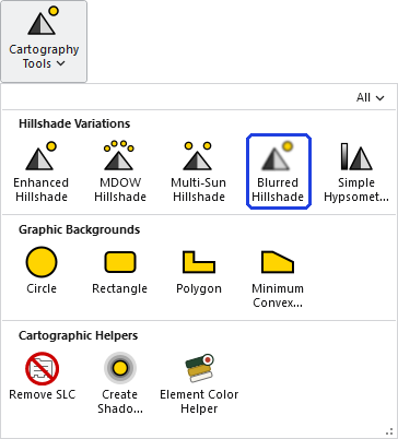
The tool opens from the Cartography group of the Wildlife and Forestry Tools ribbon tab or from the Cartography Tools toolset of the Jenness Enterprises toolbox.
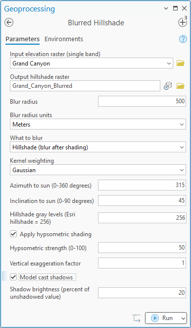
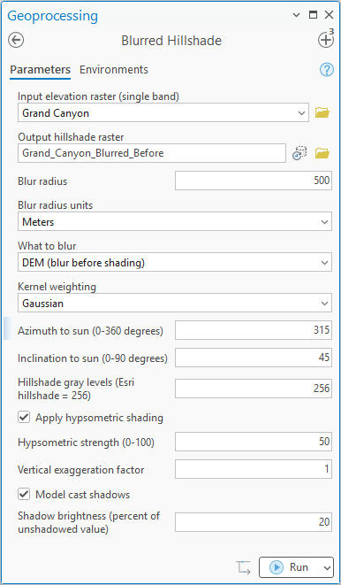
Choose the DEM and the output name. The blur settings come next: the radius, its units, what to blur and the kernel. The sun azimuth and inclination, the number of levels, hypsometric shading, vertical exaggeration and cast shadows follow, exactly as in the Enhanced Hillshade. The Elevation units row is offered only when the tool cannot tell what the elevation units are; when the DEM declares its vertical units, or is in geographic coordinates, Pro hides the row, as in the pane above. Your last choices are remembered with the project.
The output is a 16-bit integer raster from 0 to one less than the number of gray levels, NoData where the DEM is NoData and at its edge, with statistics, a histogram and bilinear pyramids already built and a black-to-white stretch applied on arrival (or, at 32 or fewer gray levels, unique values, one gray for each level).
Environment settings
By default the output matches the input DEM exactly. Processing Extent, Snap Raster, Cell Size and Output Coordinate System are honored as finishing steps applied to the computed hillshade, so the blur and the shading are always computed from the full-resolution DEM and the finished raster is then clipped, resampled or reprojected. The Mask environment is not honored, and pyramids are always built with bilinear resampling.
ModelBuilder
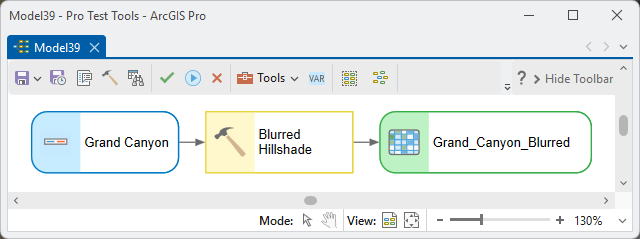
In a model the tool takes one input, the DEM, and produces one output, the blurred hillshade raster. The blur and the shading both happen inside the tool.
Parameters
| Label | Explanation | Data type |
|---|---|---|
| Input elevation raster (single band)Required · in_raster | The DEM. Must be single band; projected or geographic. Choose a layer from the map or browse to a dataset. | Raster Layer |
| Output hillshade rasterRequired · out_raster | The blurred hillshade (integer, 0 to one less than the number of gray levels). NoData where the DEM is NoData and at its outer edge. A name is suggested from the input. | Raster Dataset |
| Elevation unitsOptional · elev_units | Meters or Feet. Read from the DEM's vertical coordinate system when it has one; geographic DEMs are assumed to be in meters. In both cases the row is hidden in the dialog; you are asked only when the DEM does not say. | String |
| Blur radiusRequired · blur_radius | How far the blur reaches around each cell, in the units below. Larger is blurrier. The default is 10. | Double |
| Blur radius unitsRequired · radius_units | Cells, Meters, Kilometers, Feet or Miles. Ground units are converted to cells from the cell size, per row on the spheroid for geographic DEMs. | String |
| What to blurRequired · blur_target | DEM (blur before shading), the default, or Hillshade (blur after shading), as described above. | String |
| Kernel weightingRequired · kernel | Average (equal weights, the Focal Statistics recipe and the original method; the default) or Gaussian (sigma of half the radius, truncated at the radius; a little smoother). | String |
| Azimuth to sun (0-360 degrees)Required · azimuth | The compass direction of the sun. The default is 315. | Double |
| Inclination to sun (0-90 degrees)Required · altitude | The height of the sun above the horizon. The default is 45. | Double |
| Hillshade gray levels (Esri hillshade = 256)Required · levels | The number of gray levels; output values run from 0 to one less than this number. 32 or fewer adds a raster attribute table. | Long |
| Apply hypsometric shadingOptional · use_hypso | Darkens low elevations by the strength below. Off by default. | Boolean |
| Hypsometric strength (0-100)Optional · hypso_strength | At strength s, the brightness multiplier runs from (100 − s) percent at the lowest elevation to 100 percent at the highest. The default is 50. | Long |
| Vertical exaggeration factorOptional · vert_exag | Multiplies the elevations before shading. The default is 1. | Double |
| Model cast shadowsOptional · model_shadows | Dims ground hidden from the sun to the brightness below. Cast by the generalized terrain when the DEM is blurred first; softened by the blur when the hillshade is blurred after. Off by default. | Boolean |
| Shadow brightness (percent of unshadowed value)Optional · shadow_dim | What a shadowed cell keeps of its unshadowed value. The default is 20. | Double |
Python
import arcpy
arcpy.ImportToolbox(r"C:\path\to\JennessEnterprisesTools.pyt")  # your install path
# A 250-meter Gaussian blur of the DEM before shading.
arcpy.jenness.BlurredHillshade(
    in_raster=r"C:\Project\Elev.gdb\DEM",
    out_raster=r"C:\Project\Elev.gdb\DEM_Blurred",
    elev_units="Meters", blur_radius=250, radius_units="Meters",
    blur_target="DEM (blur before shading)", kernel="Gaussian",
    azimuth=315, altitude=45, levels=256)
# The other target string: "Hillshade (blur after shading)".
Recommended citation
Credits and references
By Jeff Jenness, Jenness Enterprises (www.jennessent.com). A new tool, grown from the blurred-hillshade lab exercise. The gradient is Horn's (1981).
- Brassel, K. 1974. A model for automatic hill-shading. The American Cartographer 1:15–27. doi.org/10.1559/152304074784107818
- Buckley, A., and D. Barnes. 2004. ArcGIS cartography: creating advanced effects for cartography in ArcMap. Technical session, 2004 Esri International User Conference, San Diego, California. content.esri.com/mappingcenter2007/resources/presentations/uc04_creatingadvancedeffectswitharcmap.pdf Accessed on September 30, 2026.
- Horn, B. K. P. 1981. Hill shading and the reflectance map. Proceedings of the IEEE 69:14–47. doi.org/10.1109/PROC.1981.11918
- Jenness, J. Raster lab 13: Hillshades with Swiss Method effects in ArcGIS Pro; Blurring the hillshade. Lab exercise video, GIS training courses, Jenness Enterprises. youtu.be/SJ6S0KgKlJQ
Licensing information
Works at every ArcGIS Pro license level (Basic, Standard, Advanced). No extension licenses are required; the blur, the shading and the shadows are computed internally, without Spatial Analyst.
Related tools and pages
- About Hillshades and the Swiss Method — the five tools compared.
- Enhanced Hillshade — the same tool without the blur.
- MDOW Hillshade — four suns, weighted by aspect.
- Multi-Sun Hillshade — a weighted average of suns you place.
- Simple Hypsometric Shading — the hypsometric effect as an adjustable group layer.
- Projecting Rasters — this tool works on geographic DEMs directly; if you project a DEM first, use bilinear interpolation.