

Simple Hypsometric Shading
Summary
Creates a group layer that drapes a DEM, drawn in a black-to-white stretch at a transparency you choose, over an existing hillshade, for the atmospheric-perspective effect of the Swiss method: the low country darkens and the high country stays bright. No new dataset is written. The group layer simply references the two rasters you already have, so everything about it stays editable afterward: the transparency, the color ramp, the stretch, the layer blend mode and the layer order. Use it when you already have a hillshade you like and want the effect as a live layer rather than baked into a file.
The idea
Seen from above, the low country of a real landscape is farther away and seen through more air, so its relief looks softer and less contrasty than the peaks. Brassel (1974) made this one of the three components of his automated Swiss method: he strengthened the contrast of the shading on the heights, reduced it in the lowlands, and slightly darkened the low country. The lab exercise does this with nothing but layers. Put the hillshade at the bottom. Put the DEM above it, symbolized with a black-to-white color ramp on a minimum-to-maximum stretch, so the lowest cell is black and the highest is white. Make the DEM 50 percent transparent. The hillshade shows through, darkened in the valleys and untouched on the summits, and the picture gains a sense of depth.
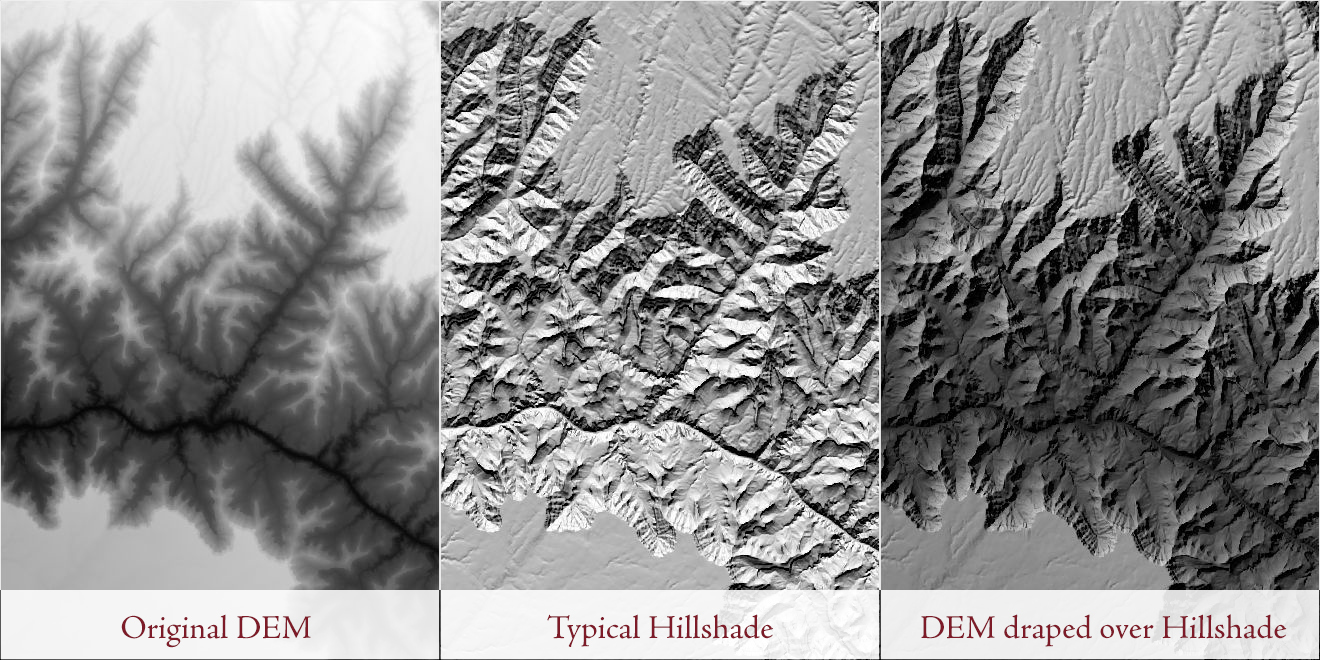
That recipe is exactly what the tool builds. It takes the DEM and the hillshade, composes a group layer with the DEM on top in a black-to-white minimum-to-maximum stretch at the transparency you set, and adds the group to the map. The hillshade can be anything: the Enhanced, MDOW, Multi-Sun or Blurred hillshade, Esri's own, or any raster you want beneath the elevation tint.
Layer blend modes
The DEM layer can also be given any of ArcGIS Pro's layer blend modes, which change how its pixels combine with the hillshade beneath. Normal is plain transparency. Multiply darkens by the product of the two layers, so the result at each cell is at least as dark as the darker layer; the lab suggests it with the DEM transparency turned down to a low number or zero. Darken keeps whichever layer is darker. Luminosity takes the brightness from the DEM and the color from what lies beneath. With the tool's black-to-white DEM over a gray hillshade there is no color on either side, so it gives the same picture as Normal. The difference shows when you give the DEM a color ramp: Normal tints the hillshade with the colors of the ramp, while Luminosity keeps only how light or dark those colors are and takes its color from the gray hillshade beneath, so the picture stays gray. Those four often work well for hypsometric shading; the full list of Pro's blend modes is offered, and since the blend mode is an ordinary layer property you can change it afterward by selecting the DEM layer and using Layer Blend on the Raster Layer ribbon tab.
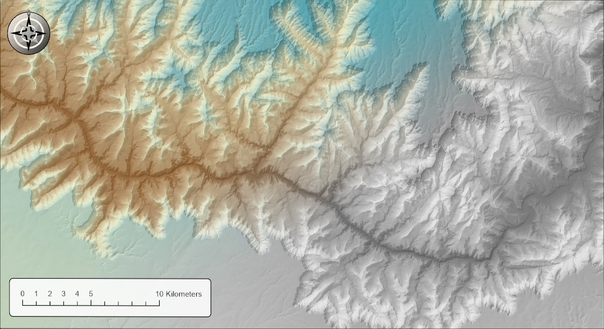
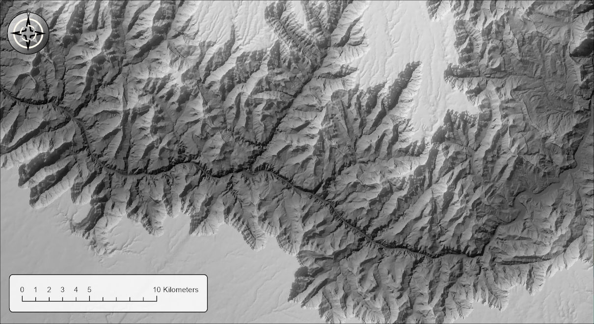
The three figures below are the same group layer, the DEM at 40 percent transparency over the same hillshade, with only the blend mode changed.
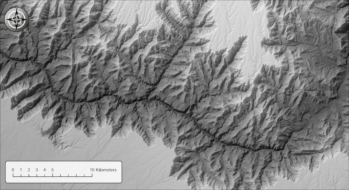
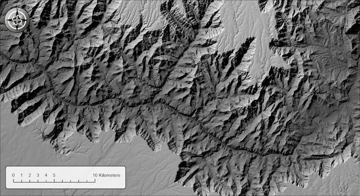
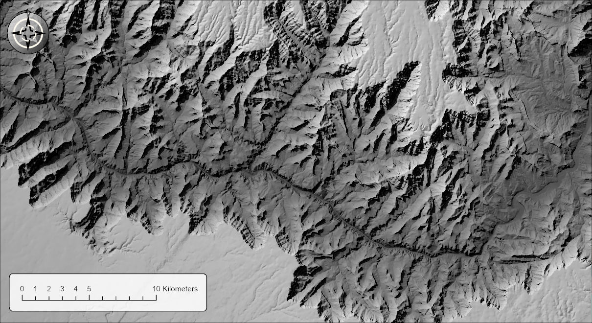
The last figure shows what Luminosity does when the DEM is in color. The DEM is drawn in a color ramp, partially transparent, over a hillshade, and the blend mode runs from Normal in the upper left corner to Luminosity in the lower right.
Adjusting the result
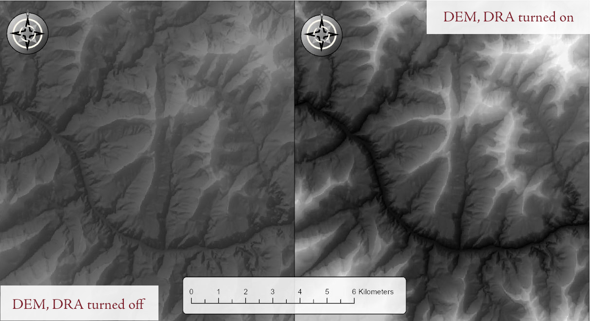
Because the output is a pair of ordinary layers, every refinement in the lab exercise is still available. Slide the DEM's transparency. Swap the black-to-white ramp for a terrain ramp to get an elevation-tinted relief map instead of a gray one. Brighten the hillshade or raise its contrast in the Raster Layer tab's Enhancement box. And if your DEM extends far beyond your map, so that the black-to-white ramp is stretched across elevations you cannot see and the visible part of the map is all one gray, turn on Dynamic Range Adjustment (DRA) in the Rendering group of the Raster Layer tab; the ramp is then stretched across the elevations in view, and the effect comes back. The lab's example is a DEM of the whole continental United States, stretched from −111 to 4,412 m, viewed on a patch that spans 2,119 to 2,315 m, where the hypsometric shading is invisible until DRA is turned on.
The alternative: bake it in
The same effect at full control is available inside the four hillshade tools as the Apply hypsometric shading option, which multiplies the hillshade values by an elevation-dependent factor and writes the result into the output raster. That is the choice when you want a single finished raster to hand to someone else or to use in another program. This tool is the choice when you want to keep adjusting.
A tour of the dialog
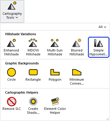
The tool opens from the Cartography group of the Wildlife and Forestry Tools ribbon tab or from the Cartography Tools toolset of the Jenness Enterprises toolbox.
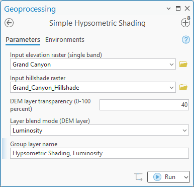
Choose the DEM and the hillshade, from the map or from disk. Set the DEM layer transparency: 0 hides the hillshade entirely under an opaque DEM, 100 hides the DEM; 50, the default, gives an even blend. Pick a Layer blend mode if you want one, and accept or change the suggested Group layer name. The tool only creates a group layer that holds two layers of rasters you already have, so the name is a layer name and not a dataset name, and none of the dataset naming rules apply: name it with spaces, commas or anything else you like, as in “Hypsometric Shading, Luminosity” in the pane above. The last-used transparency and blend mode are remembered with the project.
The tool writes a small layer file in the project's scratch folder that references the two rasters, and returns it as the output group layer, which Pro adds to the map when “Add output datasets to an open map” is on in the geoprocessing options. The DEM layer's legend shows the stretch, so it reads correctly in the Contents pane and on a layout. No raster is created and no geoprocessing environment applies.
Environment settings
None apply. The tool creates no dataset; it composes a layer file from the two rasters as they are.
ModelBuilder
In a model the output is a derived group layer. Downstream tools that take layers can use it, but since nothing is written to disk except the layer file, the usual reason to put it in a model is simply to add the finished group to the map at the end of a hillshade chain.
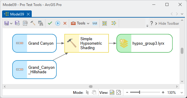
The green output element is named for a layer file,
hypso_group3.lyrx in the model above, and not for a
raster. That file is the tool's whole output. A layer file holds
no data. It records which datasets to draw and how to draw them:
here the group layer and its name, the two rasters it points to,
and the DEM layer's black-to-white stretch, transparency and blend
mode. The tool writes the file to the project's scratch folder
under a name that begins with hypso_group, numbered
so that every run gets a file of its own, and Pro makes the group
layer in the map from it. To see the group layer when you run the
model from the ModelBuilder window, right-click the output element
and choose Add To Display. The layer file depends on the two
rasters staying where they are; deleting the layer file itself
does no harm to the rasters, or to a group layer already in the
map.
Parameters
| Label | Explanation | Data type |
|---|---|---|
| Input elevation raster (single band)Required · in_dem | The DEM to drape over the hillshade. Must be single band. Choose a layer from the map or browse to a dataset. | Raster Layer |
| Input hillshade rasterRequired · in_hillshade | The hillshade to sit beneath the elevation tint, from any source. | Raster Layer |
| DEM layer transparency (0-100 percent)Required · transparency | The transparency of the whole DEM layer, 0 (opaque) to 100 (invisible). The default is 50. | Long |
| Layer blend mode (DEM layer)Optional · blend_mode | Any of Pro's layer blend modes; Normal (the default), Multiply, Darken and Luminosity often work well. Easily changed afterward on the Raster Layer tab. | String |
| Group layer nameOptional · group_name | The name of the group layer added to the map. A name is suggested from the DEM's dataset name. It is a layer name, not a dataset name, so spaces, commas and other punctuation are fine. | String |
| Output group layerDerived · out_group | The composed group layer: the symbolized DEM over the hillshade, referencing the existing rasters. | Group Layer |
Python
import arcpy
arcpy.ImportToolbox(r"C:\path\to\JennessEnterprisesTools.pyt")  # your install path
result = arcpy.jenness.SimpleHypsometricShading(
    in_dem=r"C:\Project\Elev.gdb\DEM",
    in_hillshade=r"C:\Project\Elev.gdb\DEM_Hillshade",
    transparency=50, blend_mode="Multiply",
    group_name="DEM Hypsometric Shading")
print(result.getOutput(0))   # path to the composed group .lyrx
Recommended citation
Credits and references
By Jeff Jenness, Jenness Enterprises (www.jennessent.com). A new tool, built from the hypsometric-shading lab exercise.
- Brassel, K. 1974. A model for automatic hill-shading. The American Cartographer 1:15–27. doi.org/10.1559/152304074784107818
- Jenness, J. Raster lab 10: Hillshades with Swiss Method effects in ArcGIS Pro; Hypsometric shading. Lab exercise video, GIS training courses, Jenness Enterprises. youtu.be/iymM__vq9QE
Licensing information
Works at every ArcGIS Pro license level (Basic, Standard, Advanced). No extension licenses are required; the tool only composes layers.
Related tools and pages
- About Hillshades and the Swiss Method — the five tools compared.
- Enhanced Hillshade, MDOW Hillshade, Multi-Sun Hillshade and Blurred Hillshade — hillshades to put beneath the tint, each with the baked-in alternative.