

Mahalanobis Distance Raster
Summary
Creates a raster of Mahalanobis distances measuring, for every cell, how far that cell's combination of landscape-variable values lies from a multivariate reference mean, scaled by the inverse covariance among the variables. Low values mark ground most similar to the reference conditions. If those reference conditions represent, say, the ideal habitat for some wildlife species, then the Mahalanobis raster tells you how similar every point on the ground is to that ideal habitat — a great first step toward identifying critical habitat or steering management actions. This is a similarity map of the whole landscape, and the classic multivariate habitat-modeling surface of Clark et al. (1993) and Knick and Dyer (1997).
How it works
The squared Mahalanobis distance for a cell is the quadratic form D² = (x − μ)′ Σ⁻¹ (x − μ), where x is the cell's vector of landscape-variable values, μ is the mean vector, and Σ⁻¹ is the inverse covariance matrix (bold indicates a vector or matrix, non-bold a single number). The computation processes the rasters in manageable blocks of cells rather than loading everything into memory at once, so it won't run out of memory no matter how large the rasters are or how many variables you use — and it needs no Spatial Analyst license.
The landscape variables
Variables can be rasters (cell values are always used, never attribute-table values) and/or polygon feature classes with a numeric field, which are rasterized to the analysis grid. A multiband raster automatically expands to one variable per band, and a Bands to exclude table lets you drop specific bands. At least one raster is required — it sets the analysis grid's cell size, coordinate system, and extent (adjustable through the environments).
Three sources for the reference statistics
Calculate directly from sample point features — the common wildlife case: the landscape variables are sampled at your animal locations (optionally only the selected ones), and the mean vector and covariance matrix are computed from those samples. Points outside the landscape data, or on NoData cells, are excluded and reported.
Categorical raster — the reference sample is every cell of a categorical raster belonging to a chosen category. If the raster has an attribute table, pick any of its fields as the Category attribute field and choose the category from that field's values — the tool then gathers every matching cell value automatically. Many classified rasters describe the same cells at several resolutions: a Landfire EVT raster, for example, carries both the fine-grained EVT_NAME (“Rocky Mountain Aspen Forest and Woodland”) and the broad EVT_LF (“Tree”), and choosing EVT_LF = Tree sweeps in every one of the dozens of tree-type cell values in one step. Leave the field blank to enter the numeric cell value directly instead — the right choice for a raster with no attribute table. Scripts and models may use either form: pass the field and category value exactly as the dialog does, or pass literal cell values (see the Python section).
Existing tables — a previously saved mean vector and covariance matrix, from this tool's optional table outputs or from Calculate Statistical Matrices. The variable order is validated against the tables' stored order.
The Cell value sampling option controls how raster values are read at sample points (and how rasters that don't align to the analysis grid are resampled): Exact (nearest cell) or Interpolated (bilinear). Bilinear is more appropriate for continuous surfaces like elevation; exact is right for categorical rasters — interpolation should never be used on nominal (unordered) categories.
Three flavors of output
All three are functions of the same per-cell squared distance:
| Output value | What it is |
|---|---|
| Squared distance (D²) | The quadratic form itself — the quantity traditionally mapped in ecological and habitat Mahalanobis models, and the input required by the chi-square transform. |
| Distance (D) | The square root of D²: the literal Mahalanobis distance, analogous to Euclidean distance. |
| Chi-square p-value | The upper-tail probability P(χ² > D²) with degrees of freedom equal to the number of variables: a 0 to 1 similarity score where values near 1 indicate a cell closely matching the reference conditions. See the degrees-of-freedom note on the About page. |
Inverting the covariance
Standard (inverse) is the ordinary matrix inverse — fast, exact, and the right choice in almost all cases. It fails if the covariance matrix is singular, which usually means a variable has no variance (all values identical) or two variables are perfectly correlated. Pseudo-inverse (SVD), the Moore-Penrose pseudo-inverse, returns a stable least-squares inverse instead of failing when variables are strongly collinear — though it can mask redundant variables. The tool reports the covariance condition number; very large values indicate nearly collinear variables (the correlation-matrix output is the natural way to hunt down which ones).
Saving the statistics for reuse
Four optional checkboxes also write the computed mean vector, covariance, inverse covariance, and correlation tables, auto-named from the output raster. The mean and covariance pair is what the Existing tables source reads back — compute the statistics once from your best sample, then apply them to other landscapes, other years, or the at Points tool, without resampling.
Environments
The tool honors the Output Coordinate System, Cell Size, Processing Extent, Snap Raster, and Mask environments, which together control the analysis grid. Other geoprocessing environments do not affect it.
Scenario 1: statistics from animal locations
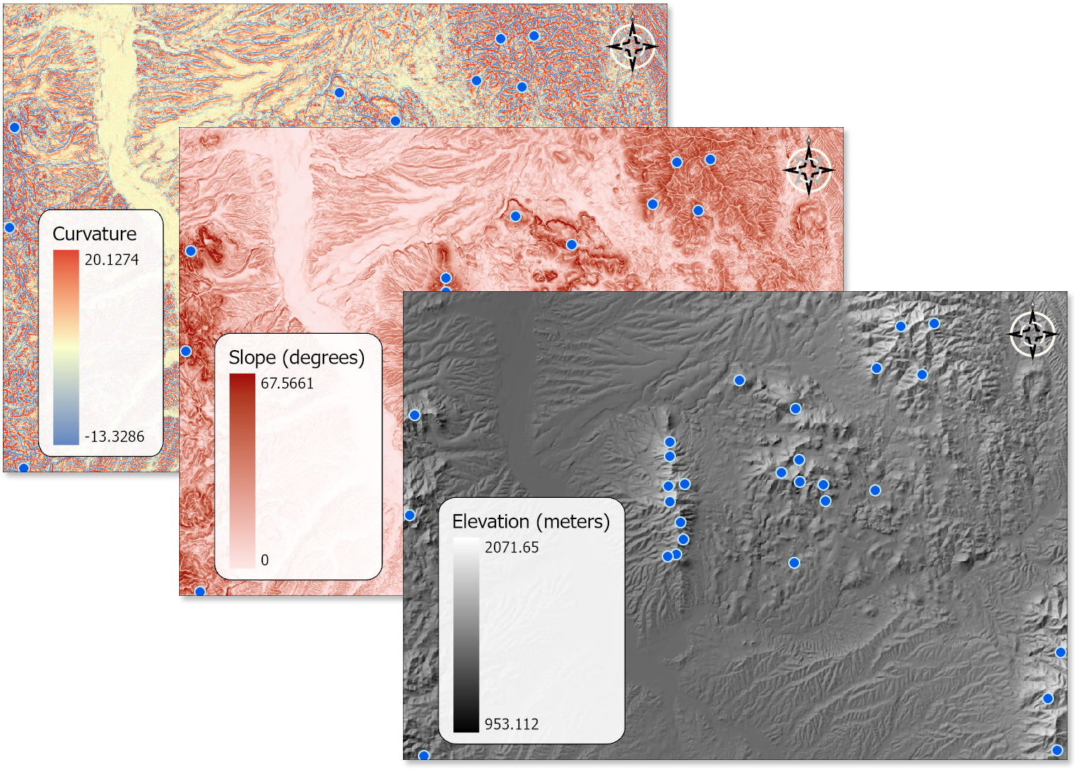
The classic wildlife case. We have locations recorded for some animal we are interested in, and we can estimate the “ideal” habitat as that which is most similar to the mean elevation, slope and landscape curvature observed at those animal locations. Just as important, the model also takes advantage of the covariance among these variables at those locations: if our animal tends to use steep slopes at low elevations and shallow slopes higher up, that relationship is baked into the covariance matrix, and the distances honor it — a cell with a typical elevation and a typical slope, but in an atypical combination, still scores as dissimilar.
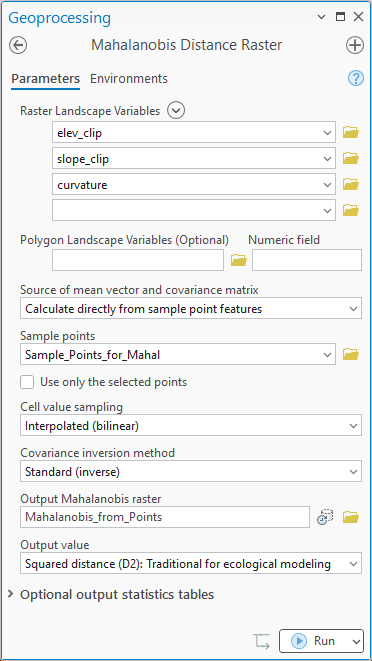
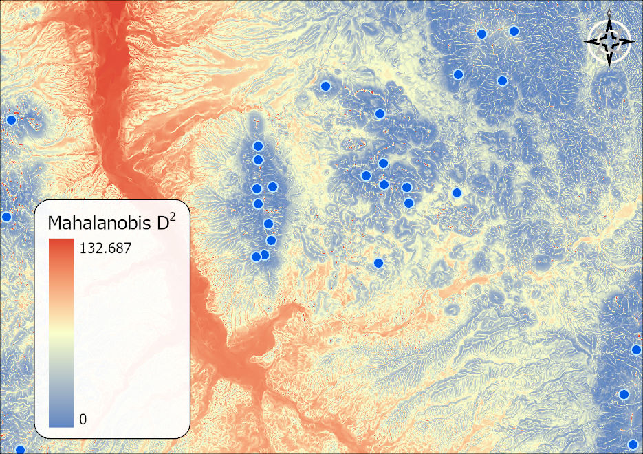
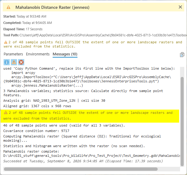
Points that don't lie within the analysis area are handled for you: any point falling outside the extent of one or more landscape rasters (or on a NoData cell) is automatically excluded from the statistics, and the analysis report tells you exactly how many were dropped and how many were used:
Scenario 2: statistics from a categorical raster
Now suppose that instead of animal locations we have a categorical raster that includes a category we care about. Here we use the Landfire Existing Vegetation Type dataset, symbolized by its EVT subclass field, and ask how similar the landscape is to the ground classified as Evergreen open tree canopy — calculating D² from the same three variables as before. The reference sample is every cell of that category (the analysis report tells you how many cells of the categorical raster matched), and the mean and covariance describe the terrain that vegetation type occupies.
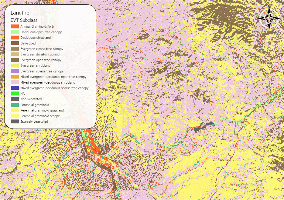
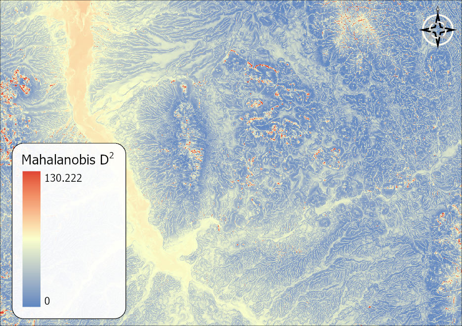
The first assumption in this example is that Landfire is categorized correctly — and you should weigh this same assumption yourself if you are using a similarly-modeled categorical raster of your own. It is a bigger assumption than it sounds, because Landfire's vegetation map is itself a model: a remote-sensing classification with its own error rate, which varies from class to class. That makes our Mahalanobis surface a second-level model, a model built on top of another model, and errors propagate quickly when you stack models this way. Every misclassified cell smuggles the wrong terrain into our reference sample, nudging the mean and covariance away from the true conditions of the vegetation type — and then every cell of the output inherits statistics contaminated by those errors. The reliabilities compound roughly multiplicatively: a classification that is 80% right, feeding a habitat model that would be 80% faithful given perfect input, leaves something closer to a 64% model, not an 80% one. None of this makes the approach invalid — it makes the output an approximation whose uncertainty is inherited from Landfire's, and worth interpreting with that in mind.
The second assumption is that the landscape variables we chose are relevant to this vegetation type, and sufficient to model it. Elevation, slope and curvature say nothing about soils, precipitation, aspect, or fire history — all of which shape where evergreen canopy actually grows. Should we have included more or different variables? That question has no automatic answer; it is an ecological judgment the tool cannot make for you.
ModelBuilder
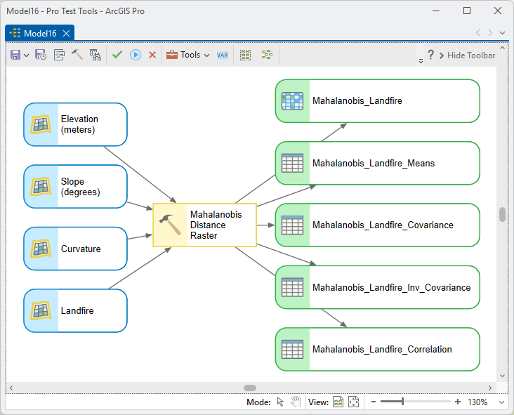
The output raster chains onward like any raster — to the Chi-Square Transform for a 0 to 1 similarity-score surface, to a Reclassify for candidate-habitat classes, or into corridor modeling. The optional statistics tables are also model outputs, so one model can compute the statistics and fan them out to several downstream Mahalanobis runs.
Parameters
| Label | Explanation | Data type |
|---|---|---|
| Raster Landscape VariablesRequired · raster_vars | The raster datasets defining the multivariate space; cell values are used, never attribute-table values. Multiband rasters expand to one variable per band. At least one raster is required. | Raster Layer (multiple) |
| Polygon Landscape VariablesOptional · poly_vars | Rows of polygon feature class + numeric field, rasterized to the analysis grid. Polygon variables follow the rasters in covariance order. | Value Table |
| Bands to excludeOptional · exclude_bands | Rows of multiband raster + 1-based band number to drop. | Value Table |
| Source of mean vector and covariance matrixRequired · stats_source | Sample point features, categorical raster, or existing tables. Choose the source first; the relevant inputs below enable accordingly. | String |
| Sample pointsOptional · points | The reference points (point-features source only). | Feature Layer |
| Use only the selected pointsOptional · use_selected | Restrict the statistics to the layer's active selection. | Boolean |
| Categorical rasterOptional · cat_raster | The raster whose matching cells form the reference sample (categorical source only). | Raster Layer |
| Category attribute fieldOptional · cat_field | A field from the raster's attribute table naming the categories the way you want to choose them (Landfire's EVT_NAME or EVT_LF, say); leave blank to enter a literal cell value instead. | Field |
| Category valueOptional · cat_value | The category whose cells form the reference sample — a dropdown of the chosen field's values, with every matching cell value gathered automatically. With no field, literal cell value(s), semicolon-separated for several (“3;4;5”). | String |
| Mean vector tableOptional · mean_table | A saved mean vector (existing-tables source only). | Table View |
| Covariance matrix tableOptional · cov_table | A saved covariance matrix; its stored variable order validates the variable list. | Table View |
| Cell value samplingOptional · sample_method | Exact (nearest cell) or Interpolated (bilinear); see above. | String |
| Covariance inversion methodRequired · inversion | Standard (inverse) or Pseudo-inverse (SVD); see above. | String |
| Output Mahalanobis rasterRequired · out_raster | The output raster; defaults to Mahalanobis in the current workspace, auto-incremented. | Raster Dataset |
| Output valueRequired · out_type | Squared distance (D²), Distance (D), or Chi-square p-value. | String |
| Generate / save statistics tablesOptional · gen_mean…save_corr | Checkbox-and-output pairs for the mean vector, covariance, inverse covariance, and correlation tables, auto-named from the raster name (_Means, _Covariance, _Inv_Covariance, _Correlation). | Boolean + Table |
Python
A D² raster from three rasters in the active map, with statistics from a sample-point layer, saving all four statistics tables:
import arcpy
arcpy.ImportToolbox(r"C:\path\to\JennessEnterprisesTools.pyt")  # your install path
out_gdb = r"C:\Project\Mahalanobis.gdb"
arcpy.jenness.MahalanobisRaster(
    raster_vars="elev_clip;slope_clip;curvature",
    sample_method="Interpolated (bilinear)",
    stats_source="Calculate directly from sample point features",
    points="Sample_Points_for_Mahal",
    inversion="Standard (inverse)",
    out_raster=out_gdb + r"\Mahalanobis",
    out_type="Squared distance (D2): Traditional for ecological modeling",
    gen_mean=True,  save_mean=out_gdb + r"\Mahalanobis_Means",
    gen_cov=True,   save_cov=out_gdb + r"\Mahalanobis_Covariance",
    gen_invcov=True, save_invcov=out_gdb + r"\Mahalanobis_Inv_Covariance",
    gen_corr=True,  save_corr=out_gdb + r"\Mahalanobis_Correlation")
Categorical-raster statistics work the same way in a script as in the dialog: pass the attribute field and category value, and the tool gathers every matching cell value itself — the script never needs to look up the codes:
arcpy.jenness.MahalanobisRaster(
    raster_vars="elev_clip;slope_clip;curvature",
    stats_source="Categorical raster",
    cat_raster="Landfire",
    cat_field="EVT_LF",
    cat_value="Tree",
    inversion="Standard (inverse)",
    out_raster=out_gdb + r"\Mahalanobis_Tree",
    out_type="Squared distance (D2): Traditional for ecological modeling")
Alternatively, skip the field and supply literal cell value(s) yourself — a single value, or several separated by semicolons, every listed value joining the reference sample:
    # ...same call, but with:
    cat_field=None,
    cat_value="7016;7019;7023",
Recommended citation
Credits and references
By Jeff Jenness, Jenness Enterprises (www.jennessent.com), ported from his ArcView Mahalanobis Distances extension and the ArcMap Land Facet Corridor Tools.
- Clark, J. D., J. E. Dunn, and K. G. Smith. 1993. A multivariate model of female black bear habitat use for a geographic information system. Journal of Wildlife Management 57:519–526. doi.org/10.2307/3809276
- Farber, O., and R. Kadmon. 2003. Assessment of alternative approaches for bioclimatic modeling with special emphasis on the Mahalanobis distance. Ecological Modelling 160:115–130. doi.org/10.1016/S0304-3800(02)00327-7
- Knick, S. T., and D. L. Dyer. 1997. Distribution of black-tailed jackrabbit habitat determined by GIS in southwestern Idaho. Journal of Wildlife Management 61:75–85. doi.org/10.2307/3802416
- Mahalanobis, P. C. 1936. On the generalised distance in statistics. Proceedings of the National Institute of Sciences of India 2(1):49–55. Reprinted 2018 in Sankhyā A 80(Suppl 1):S1–S7. doi.org/10.1007/s13171-019-00164-5
Licensing information
Works at every ArcGIS Pro license level (Basic, Standard, Advanced). No extension licenses are required — including Spatial Analyst.
Related tools and pages
- About Mahalanobis distances — theory, worked example, and the chi-square p-value discussion.
- Mahalanobis Distance at Points — the same value at point features instead of every cell.
- Calculate Statistical Matrices — compute the reference statistics once, reuse them here.
- Mahalanobis Chi-Square Transform — rescale this tool's D² output to a 0 to 1 similarity-score surface.