

Kernel Density Enhanced
Summary
Creates a kernel density surface from point features. With its defaults — the quartic kernel and the Silverman bandwidth rule — it reproduces Esri's Kernel Density tool exactly; beyond them it offers seven kernel shapes, an explicit planar/geodesic distance choice, and three kinds of output cell value, including a proportion-under-curve surface which can be used to generate home range polygons that represent a consistent activity level from the observed locations. For example, we might consider the region with the highest 10% of activity as the core area, and the region with 90% of activity as the home range or territory. Setting thresholds based on activity level allows us to compare home ranges among different individuals using a consistent standard. And unlike the Esri tool, this tool needs no Spatial Analyst license.
What it builds
Each input point is replaced by a smooth, finite-support kernel — a bell of density that adds weight to nearby cells out to the search radius (bandwidth) and drops to zero beyond it — and the overlapping bells are summed into one surface. Such surfaces are the standard estimator of animal utilization distributions (Worton 1989) and of the density of any mapped features. An optional population field weights each point (a count of animals at a colony, say); otherwise every point counts as 1 and is therefore equally weighted.
Three kinds of cell value
Densities — points per your chosen area unit (square kilometers, hectares, acres…): the classic Esri behavior. Expected counts — the expected number of points per cell; the cell values sum to the total number of input points. Proportion under curve — the cumulative proportion of the total volume under the surface, from about 0 at the outer edge to 1 at the peak: the “step farther” that makes home ranges comparable across animals, produced in a single run. Contour it at 1 − X/100 for the X% isopleth — or hand it to KD Probability Contours, which recognizes it automatically.
The seven kernel shapes
All seven kernels have finite support — they reach exactly zero at the search radius. (Infinite-tailed kernels such as the Gaussian, which never quite reach zero, are deliberately not offered because these types of kernels don't actually have a clearly defined search radius/bandwidth.) All are normalized so each point contributes the same total volume; they differ in how sharply weight falls off with distance. Quartic is the default and matches the Esri tool exactly; uniform is a flat disk (simple point density, in effect); triangular falls off linearly (a cone); Epanechnikov is a gentle, statistically efficient parabola; triweight and tricube are more sharply peaked; cosine is a raised-cosine taper.
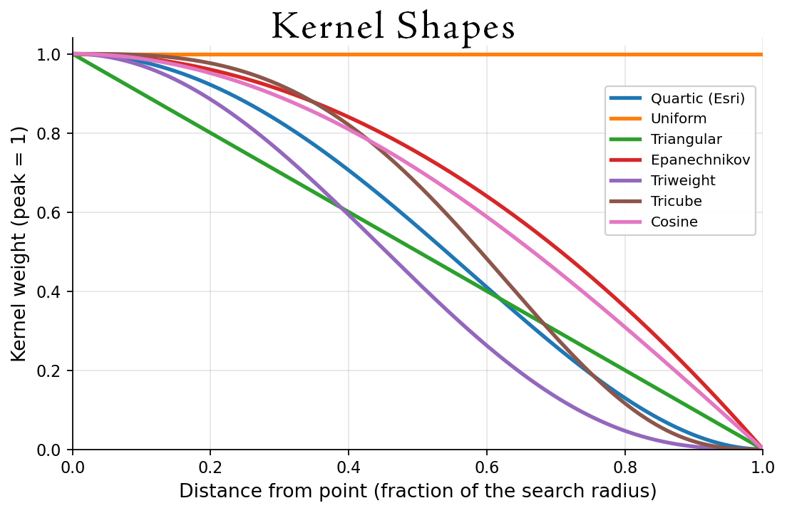
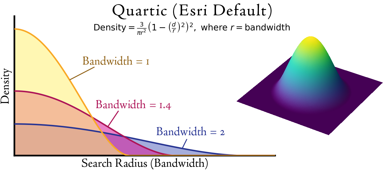
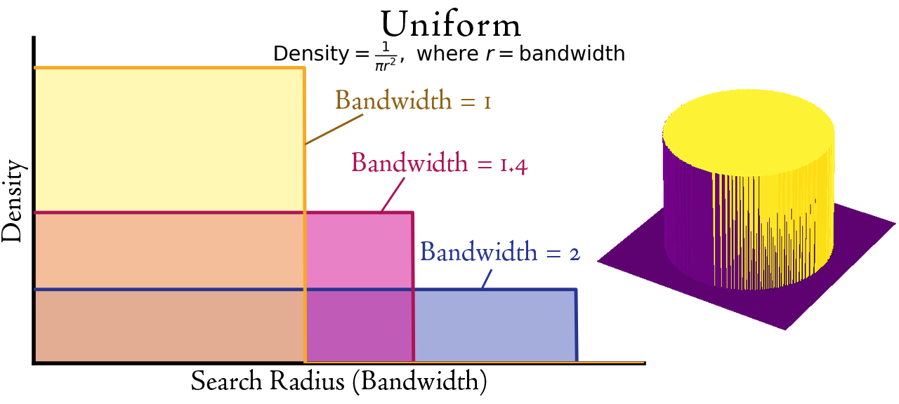
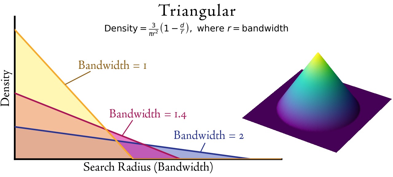
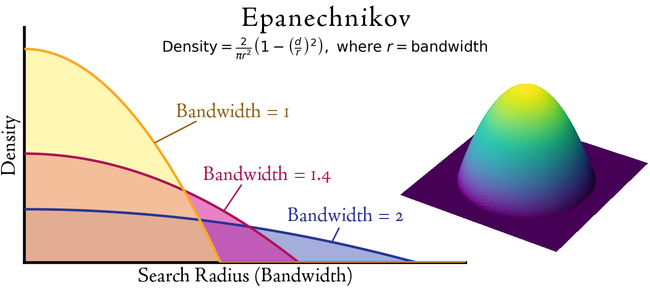
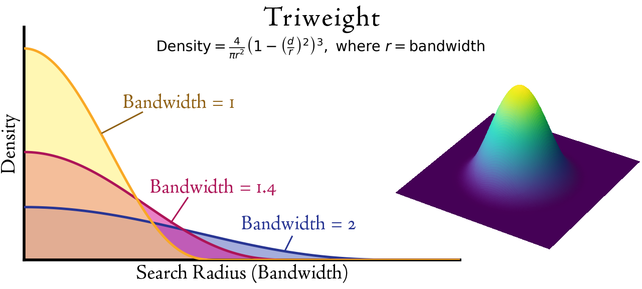
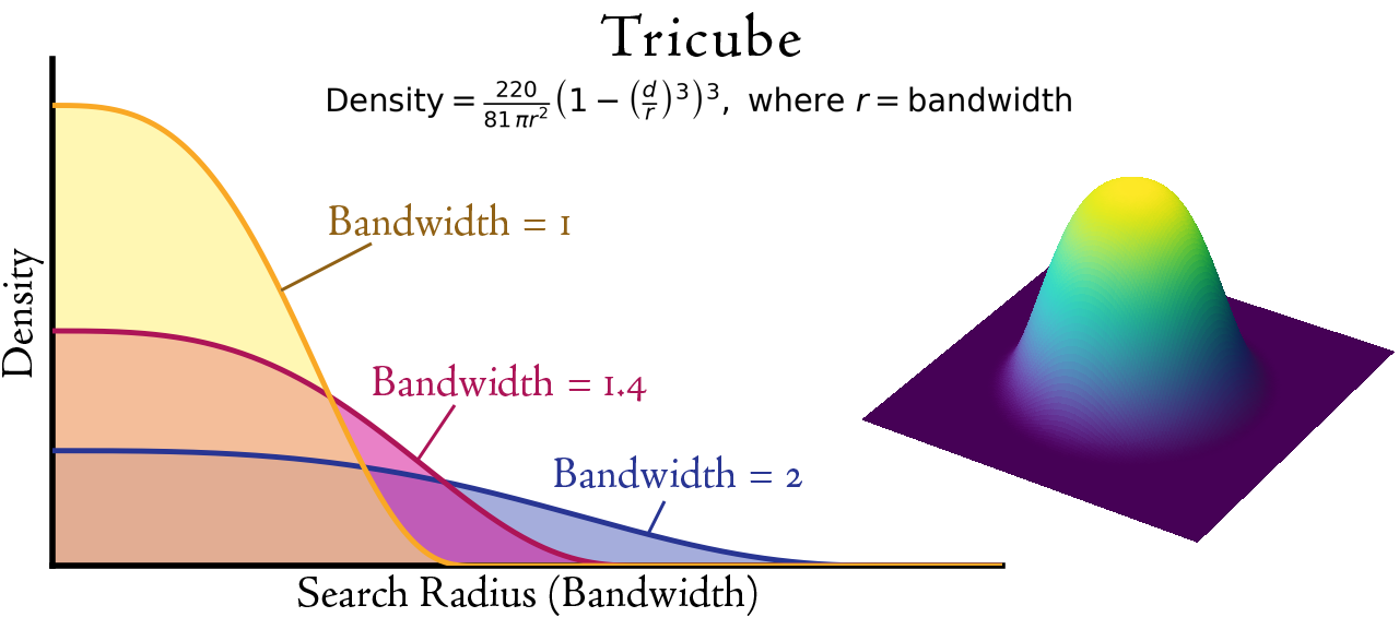
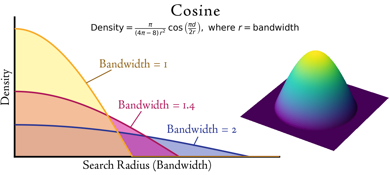
For each kernel: its density equation, the same total volume at three bandwidths (the peak drops as the bandwidth grows), and a 3-D perspective of the surface.
The search radius, and its default
The search radius is the distance at which every point's bell reaches zero — the single most consequential setting in the analysis (small = detail and fragmentation, large = smoothness and generalization). Leave it empty and the tool computes Silverman's rule of thumb, the same default as the Esri tool, from the spatial distribution of the points — including the weighted variants when a population field is used, and computed correctly for geodesic analyses of projected data. The About page's sidebar gives the formula and, more importantly, the caveat: the default is a best guess based only on where the points sit, so treat it as a starting value.
Planar or geodesic
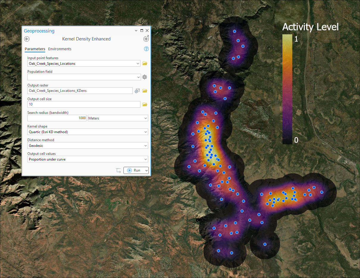
Planar measures straight-line distance in the projection's linear units; Geodesic measures true distance on the spheroid. Input in a geographic (latitude–longitude) coordinate system is always analyzed geodesically, and the choice is then locked. The output raster carries statistics and a histogram, so it renders correctly and stores the statistics with the dataset automatically — and it arrives on the map already symbolized, with a dark-purple-to-yellow density ramp at 30% transparency, so the surface reads over imagery immediately.
A tour of the dialog
A basic Esri-equivalent run needs only the points and an output name — quartic kernel, Silverman bandwidth, and the auto-filled cell size come standard. The kernel shape, distance method, output value type, and area units cover the enhancements.
ModelBuilder
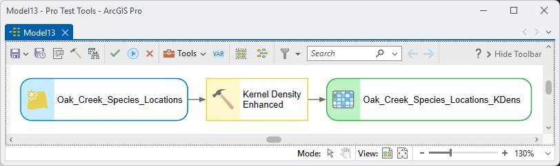
The density raster chains onward directly — and with Proportion under curve as the output value, a single model step goes from points to a surface that KD Probability Contours can turn into home-range polygons.
Parameters
| Label | Explanation | Data type |
|---|---|---|
| Input point featuresRequired · in_features | The points whose density is estimated. A layer selection is honored; geographic input is analyzed geodesically. Every point of a multipoint feature is used. | Feature Layer |
| Population fieldOptional · population_field | Optional numeric weight per point (a count, for example). NONE = every point counts as 1. | Field |
| Output rasterRequired · out_raster | The kernel density surface (single continuous band). | Raster Dataset |
| Output cell sizeOptional · cell_size | A number or an existing raster; auto-filled with the Esri default (Cell Size environment, else Snap Raster's cell, else the shorter extent side / 250). | Analysis Cell Size |
| Search radius (bandwidth)Optional · search_radius | The distance at which each kernel reaches zero. Empty = the Silverman default. | Linear Unit |
| Kernel shapeRequired · kernel | One of the seven finite-support kernels; Quartic (Esri KD method) is the default. | String |
| Distance methodRequired · distance_method | Planar or Geodesic; locked to Geodesic for geographic input. | String |
| Output cell valuesRequired · out_value | Densities, Expected counts, or Proportion under curve. | String |
| Area unitsOptional · area_unit | The area unit for the Densities output (Square kilometers, Hectares, Acres…). | String |
Environments
The tool honors Output Coordinate System (the points are projected in and the whole surface is computed there, not resampled afterward), Cell Size, Processing Extent, Snap Raster, and Mask.
The Mask is applied last, to the finished surface. With the Proportion under curve output, the proportions are computed from the whole surface first and the mask then trims them, so the cells that remain keep their true values. The same is not true of a masked Densities or Expected counts raster converted afterward: KD to Proportion Surface and KD Probability Contours can only see the cells in the raster, and treat the trimmed surface as the whole distribution. If you need both a mask and proportions, produce the proportions here in one step. A Processing Extent smaller than the surface is different: it limits the surface the tool computes, so the proportions describe only the part inside the extent.
The default extent is worth calling out as an advantage in its own right: when no Processing Extent is set, this tool automatically expands the output to the extent of the points plus the bandwidth distance, so every kernel runs all the way out to zero. Esri's Kernel Density tool only generates the surface within the extent of the points themselves, so its raster is cut off at the edges — the outermost bells sliced mid-slope — unless you remember to set an analysis extent environment yourself.
Python
A quartic density surface in points per square kilometer, with the Silverman bandwidth:
import arcpy
arcpy.ImportToolbox(r"C:\path\to\JennessEnterprisesTools.pyt")  # your install path
arcpy.jenness.KernelDensityGenerate(
    in_features=r"D:\data\telemetry.gdb\owl_fixes",
    out_raster=r"D:\data\telemetry.gdb\KD_density",
    kernel="Quartic (Esri KD method)",
    distance_method="Planar",
    out_value="Densities",
    area_unit="Square kilometers")
Recommended citation
Credits and references
By Jeff Jenness, Jenness Enterprises (www.jennessent.com).
- Silverman, B. W. 1986. Density estimation for statistics and data analysis. Monographs on Statistics and Applied Probability, Vol. 26. Chapman and Hall, London.
- Worton, B. J. 1989. Kernel methods for estimating the utilization distribution in home-range studies. Ecology 70:164–168. doi.org/10.2307/1938423
Licensing information
Works at every ArcGIS Pro license level (Basic, Standard, Advanced). No extension licenses are required — Esri's Kernel Density tool, by contrast, requires the Spatial Analyst extension.
Related tools and pages
- About kernel density analysis — the theory, from point density to probabilities.
- KD to Proportion Surface — rescale any density raster to the 0-to-1 proportion surface.
- KD Probability Contours — the home-range isopleths, drawn for you.
- About LoCoH — the local-hull road to the same utilization distribution.