

Kernel Density Probability Contours
Summary
Generates home-range probability (volume) isopleths from a kernel density surface at the standard levels — 5% to 100% in 5% steps — as contour polylines and/or polygon areas. The X% isopleth bounds the smallest area containing X% of the estimated use. For example, one reasonable way to delineate core areas and home ranges might be to single out the 95% level for the home range and the 50% level as the core. The tool recognizes what kind of raster you hand it and contours accordingly.
Two inputs, one answer
The tool automatically recognizes your input:
A kernel density raster — Esri's Kernel Density output, or the Densities or Expected counts output of Kernel Density Enhanced: the tool sorts the cell values, accumulates the volume, finds the density threshold that encloses each target percentage, and contours those thresholds.
A proportion-under-the-surface raster — from KD to Proportion Surface or Kernel Density Enhanced's Proportion under curve output: the cumulative volume is already stored in the cells, so the tool simply contours the standard proportion levels directly. These rasters are identified by a marker written into their metadata — not by guessing from the cell values, which would misfire on other 0-to-1 rasters. Isopleths from the two paths agree to within a fraction of a percent.
You may produce contour polylines, polygon areas, or both (at least one is required); the polygon boundaries coincide exactly with the polylines, and both carry the same attribute fields. Each polygon is the ground where the surface is at or above its level: a hollow inside an isopleth, a patch the animal used less than its surroundings, is left as a hole, and an isopleth that runs off the edge of the raster is closed along the edge.
Give this tool the whole surface. The tool can only see the cells in the raster, and it treats their total as the whole distribution. A density raster that was trimmed by a Mask, clipped, or cut off by a small Processing Extent is missing part of its volume, so every isopleth computed from it is a share of the trimmed surface and not of the animal's full distribution. If you need a masked proportion surface, run Kernel Density Enhanced with the mask and its Proportion under curve output: it computes the proportions from the whole surface and trims them afterward.
The outermost isopleth, labeled 100%, is the edge of the surface itself, where the density trails off to nothing. It is drawn as a smooth closed line along the edge of the cells with a density above zero, not as a staircase of cell sides.
On a latitude/longitude raster the cells are not all the same size: they narrow toward the poles. The volume under the surface is density times cell area, so the tool needs to know what the cell values are. If they are densities, each cell is weighted by its true area. If they are expected counts, the area is already in the values, and the cells are ranked by the count a cell of average size would hold, which is their density. The tool reads the answer from the raster's metadata: Kernel Density Enhanced records what it wrote, and Esri's Kernel Density records its choice in the geoprocessing history. Only when the metadata does not say does the tool assume densities, and the Raster cell values parameter, which appears only for latitude/longitude rasters, then shows a warning so you can correct it. On a projected raster every cell has the same area and none of this matters.
Output fields
| Field | Definition |
|---|---|
| Density | The raster value contoured to produce this isopleth — a density threshold for a density input, a cumulative proportion for a proportion input. |
| Isopleth | The home-range isopleth level: the proportion (0 to 1) of the total volume enclosed by this contour (0.95 = the 95% isopleth). |
| CumProportion | 1 − Isopleth: the value at which to contour a proportion surface to reproduce this isopleth. In a shapefile output, whose field names are limited to ten characters, the field is named CumProport. |
| Label | The level as a percentage label (“95%”). |
| Primary | True for the prominent levels (5, 25, 50, 75, 95%), False for the minor ones — ready-made for a two-weight symbology. |
And the outputs arrive already symbolized that way: the primary isopleths draw as heavier dark lines and the minor levels as lighter gray ones (polygons draw hollow with the same outline weights, so the nested isopleths all stay visible).
Coordinate system behavior
Contours are generated in the raster's own coordinate system; if the Output Coordinate System environment is set, the finished polylines and polygons are reprojected to it as a last step. No other environments affect the tool.
A tour of the dialog
One input raster, two checkbox-and-output pairs — lines, areas, or both.
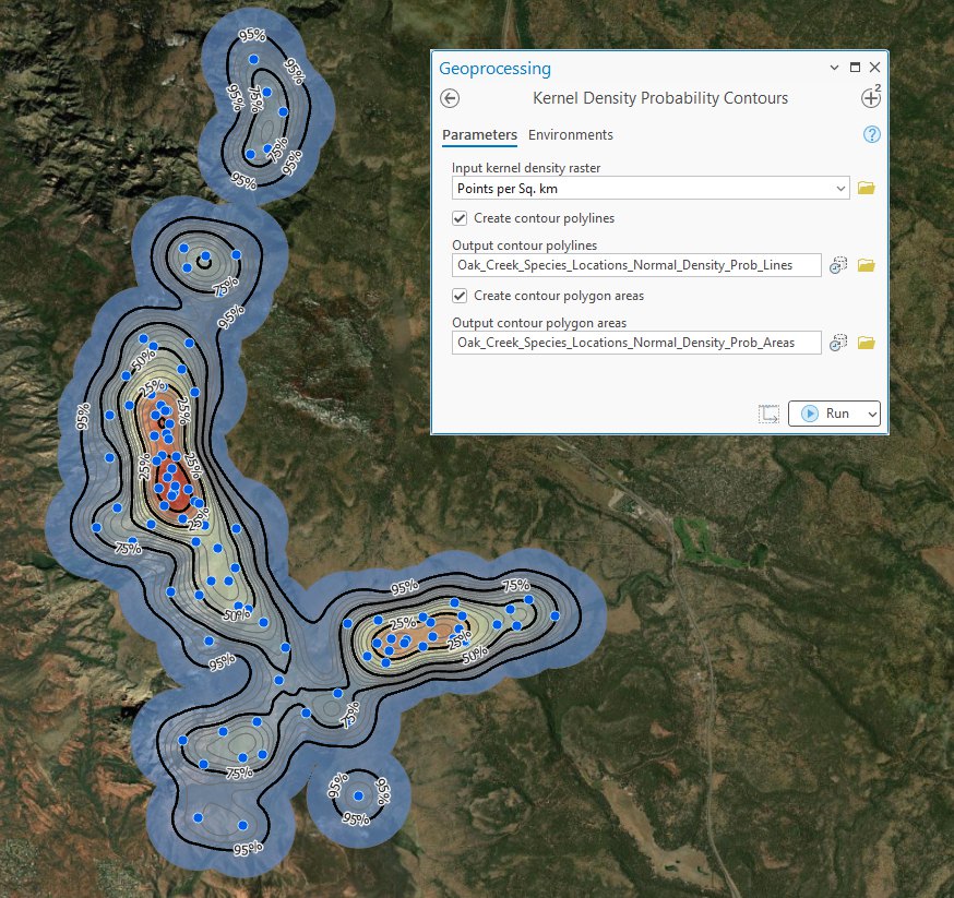
The tool holds the whole raster in memory at once, so the memory it needs grows with the number of cells. On most rasters that is no concern. On a very large one the tool may need more memory than your computer has free, and then one of two things happens: Windows starts using the disk as overflow memory and the tool slows to a crawl, or the tool stops with an out-of-memory error. There is no fixed limit; it depends on how much memory your computer has free. If a raster is too large, clip it to the area you need first.
ModelBuilder
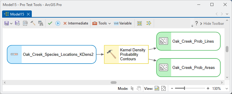
The polygon areas are the model-friendly output. As one example of how the isopleths could be used downstream, a Select on Isopleth = 0.95 might pull out a home-range polygon and Isopleth = 0.50 a core area, chaining onward to clip habitat rasters, compute areas, or compare animals — but those two levels are conventions, not the law, and any of the twenty levels can reasonably serve whatever threshold fits your analysis.
Parameters
| Label | Explanation | Data type |
|---|---|---|
| Input kernel density rasterRequired · in_raster | A kernel density raster or a proportion-under-the-surface raster; the tool detects which and contours accordingly. | Raster Layer |
| Create contour polylinesOptional · make_lines | Check to produce isopleth polylines. At least one output is required. | Boolean |
| Output contour polylinesOptional · out_lines | The isopleth contour polylines, with the fields above. | Feature Class |
| Create contour polygon areasOptional · make_polys | Check to produce the enclosed polygon areas. | Boolean |
| Output contour polygon areasOptional · out_polys | The isopleth polygon areas; boundaries coincide with the polylines. | Feature Class |
| Raster cell values (latitude/longitude rasters)Optional · value_kind | Densities or Expected counts. Shown only for a latitude/longitude raster, and filled in from the raster's metadata; Densities is assumed, with a warning, when the metadata does not say. | String |
Python
Isopleth polylines and polygon areas from a density raster:
import arcpy
arcpy.ImportToolbox(r"C:\path\to\JennessEnterprisesTools.pyt")  # your install path
arcpy.jenness.KernelDensityContours(
    in_raster=r"D:\data\telemetry.gdb\KD_density",
    make_lines=True,
    out_lines=r"D:\data\telemetry.gdb\KD_isopleth_lines",
    make_polys=True,
    out_polys=r"D:\data\telemetry.gdb\KD_isopleth_areas")
Recommended citation
Credits and references
By Jeff Jenness, Jenness Enterprises (www.jennessent.com). The volume-isopleth approach to kernel home ranges follows Worton.
- Worton, B. J. 1989. Kernel methods for estimating the utilization distribution in home-range studies. Ecology 70:164–168. doi.org/10.2307/1938423
Licensing information
Works at every ArcGIS Pro license level (Basic, Standard, Advanced). No extension licenses are required.
Related tools and pages
- About kernel density analysis — the theory behind the isopleths.
- Kernel Density Enhanced — builds the surfaces this tool contours.
- KD to Proportion Surface — the rescaling this tool recognizes automatically.
- The LoCoH tools — isopleths by local hulls instead of kernels, trimmed at the observed locations.