

About LoCoH Home-Range Analysis
This page covers the ideas shared by the three Local Convex Hull (LoCoH) tools — Standard (k), Adaptive (a), and Fixed Sphere (r) — so each tool's page can concentrate on what makes its variant different.
From locations to a home range
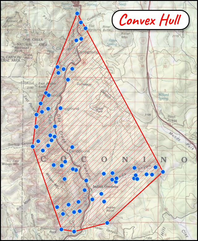
A season of telemetry gives you a cloud of locations; the home-range question is what area those locations represent. The simplest and most intuitive answer, the minimum convex polygon, treats the locations like pins in a map, and the MCP like a rubber band stretched around them. It is conservative, in the sense that it is guaranteed to capture all the land the animal actually uses for its home range (assuming you have good data of course), but it also often captures regions the animal never actually goes. You see this most when the animal is restricted to specific vegetation or topographic features, and those features extend in uneven shapes over the landscape. For example, the figure below shows the locations of a hypothetical canyon-dwelling species in Oak Creek Canyon, northern Arizona: every fix lies in the canyon system, yet the convex hull sweeps in the whole plateau above the eastern rim — miles of ponderosa pine the animal never touches — simply because the canyon bends and a convex boundary cannot bend with it. Report that polygon as the home range and you have badly overstated the area the animal actually uses, with real management consequences (the Concave Hull page follows this same example further).
A second limitation runs deeper than the shape: even a perfect boundary is only a boundary. It says nothing about how the animal used the inside — where the core areas are, which country is crossed once and which is lived in. Modern home-range analysis therefore aims at something richer: the utilization distribution, a description of where the animal spends its time. The practical form of a utilization distribution is a nested set of isopleths — polygons enclosing a stated proportion of the use. The 50% isopleth outlines the core areas; the 95% isopleth is the conventional home-range boundary, drawn so a few outlying excursions do not inflate the estimate.
Two roads to the utilization distribution
Two common methods estimate the utilization distribution from a set of locations: kernel density estimation — implemented here by our Enhanced Kernel Density tools — and this Local Convex Hull method. Both are great methods, and both are appropriate, defensible ways to estimate resource use; the choice should come from how each one applies to your particular situation, because each has its own pros and cons.
Kernel densities (usually referred to as “heat maps” outside of scientific journals) are better at estimating resource use cell by cell across a continuous raster surface — a per-cell picture of intensity that no set of polygons can match. And by definition — because of the shape of the kernel — they also estimate some level of use outside the observed range of the animal. Sometimes this is good: no season of telemetry observes every place the animal went, and the kernel's spread allows for the unobserved. Sometimes it is not.
One cool thing about the LoCoH methods is the opposite behavior: because every hull is built only from actual locations, the final isopleth polygons are trimmed right at the edge of the observed locations. That makes LoCoH better at restricting the home range where a genuine sharp boundary prevents the animal from entering — a lake next to the territory of a land-dwelling animal, say. If that animal was observed at the edge of the lake, a kernel density estimator would treat the portion of the lake near that observation as area the animal uses; LoCoH keeps the shoreline. LoCoH is also nonparametric — no bandwidth, no distributional assumption — and it degrades gracefully: as the neighborhoods grow, every variant converges to the minimum convex polygon.
How LoCoH works — a walkthrough
The LoCoH method (Getz and Wilmers 2004; Getz et al. 2007) is an interesting variation on the standard MCP approach that does reasonably well at excluding areas the animal does not use, and even distinguishes between areas with different levels of use. It generates a series of convex hulls around subsets of locations, then progressively combines them into larger polygons. The method allows you to classify regions according to how many of the points are captured, and does well at finding areas with high and low use. It also does well at capturing natural boundaries and obstacles that may exist on the landscape.
Let's walk the method through on the locations of Mexican spotted owl #6 — an owl who also stars in the lab exercises of Jeff's GIS training course. The standard MCP around all of the owl's locations looks like this:
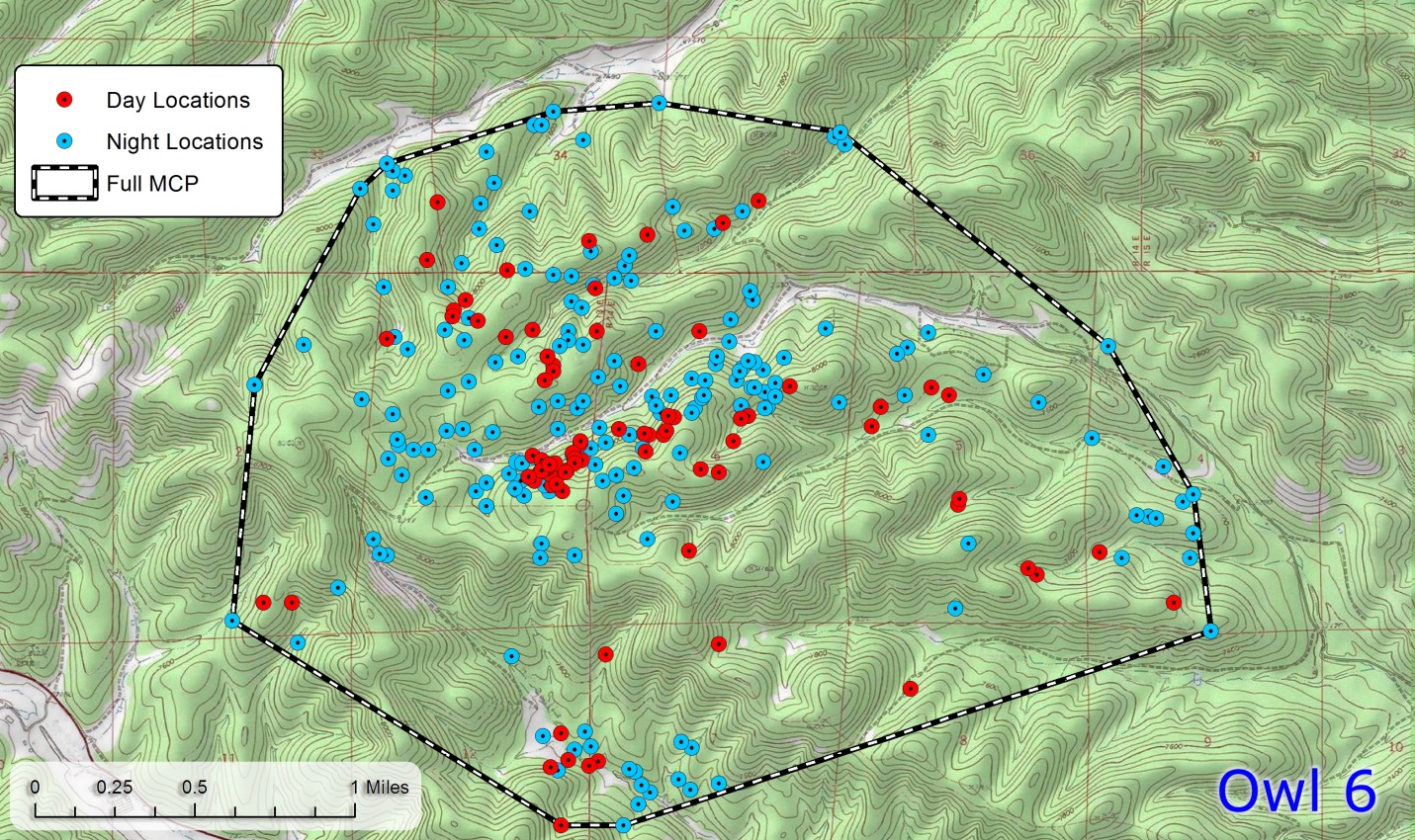
Visually we can see that some parts of this hull are used more than others, so the simple MCP is missing some important information about where the owl prefers to be. We could turn to Kernel Densities if we wanted to look for where this owl concentrates its activity, but Local Convex Hulls are another method worth trying.
The method starts with finding the k nearest neighbors to every point. You specify the value for k, and larger numbers produce output that comes closer to the original full MCP — if your value of k equals the total number of points in your dataset, you end up with exactly the full MCP above. Lower values of k classify the landscape in a much tighter range around the clusters of points.
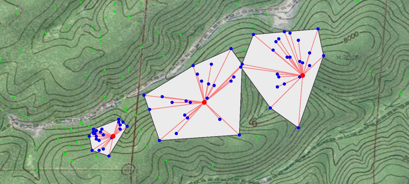
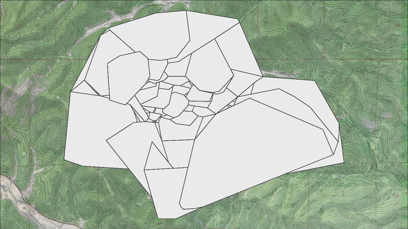
We generate a convex hull around the group of k nearest neighbors to the first point in the dataset, then repeat the process for the next point, then again for all points. For example, at k = 25, every location gets the convex hull of its nearest 25 neighbors:
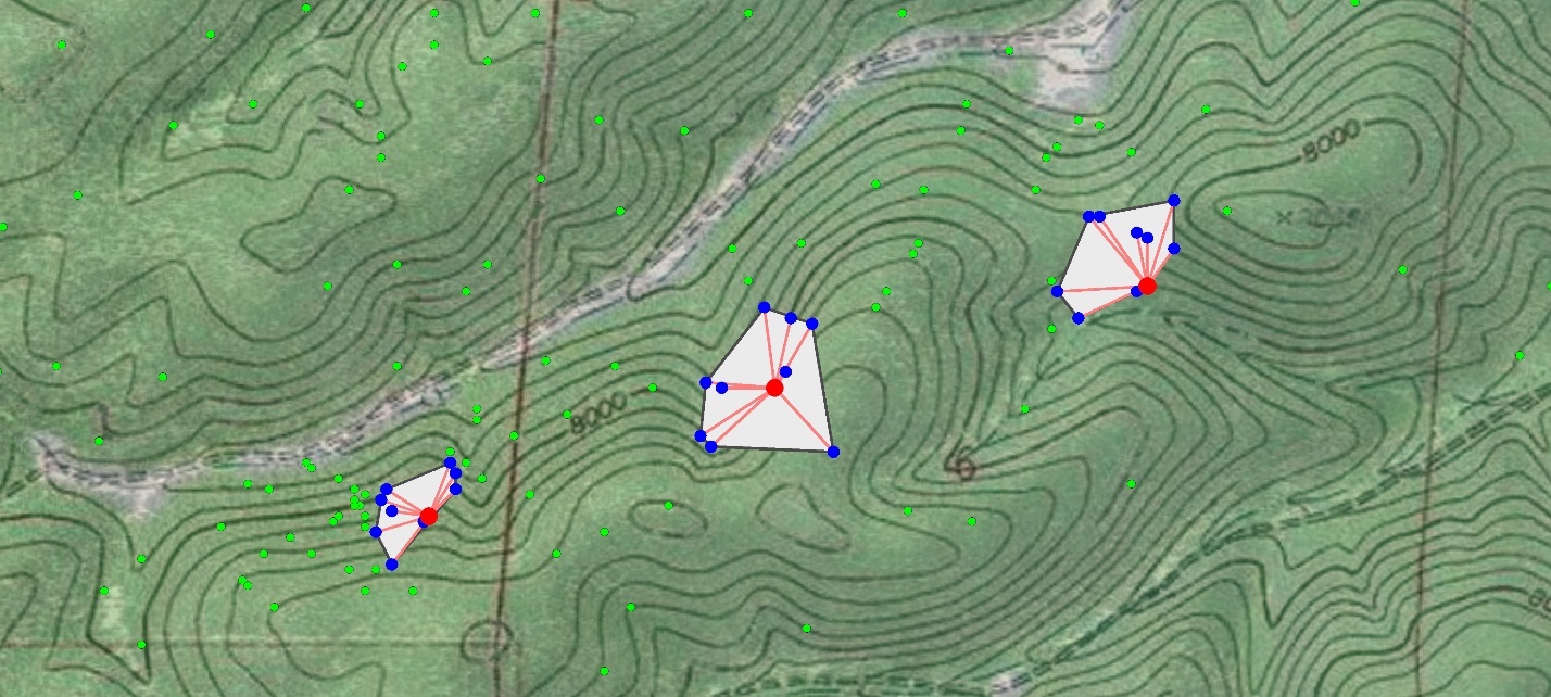
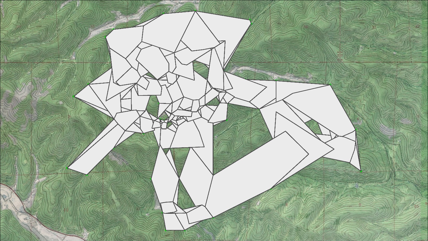
At k = 10 we would generate just as many convex hulls, but each a little smaller, because every hull encloses only the 10 points nearest its focal location:
At the end of this step we have as many convex hulls as we have points. At k = 25, the full set looks like this:
At k = 10, the hulls look like this:
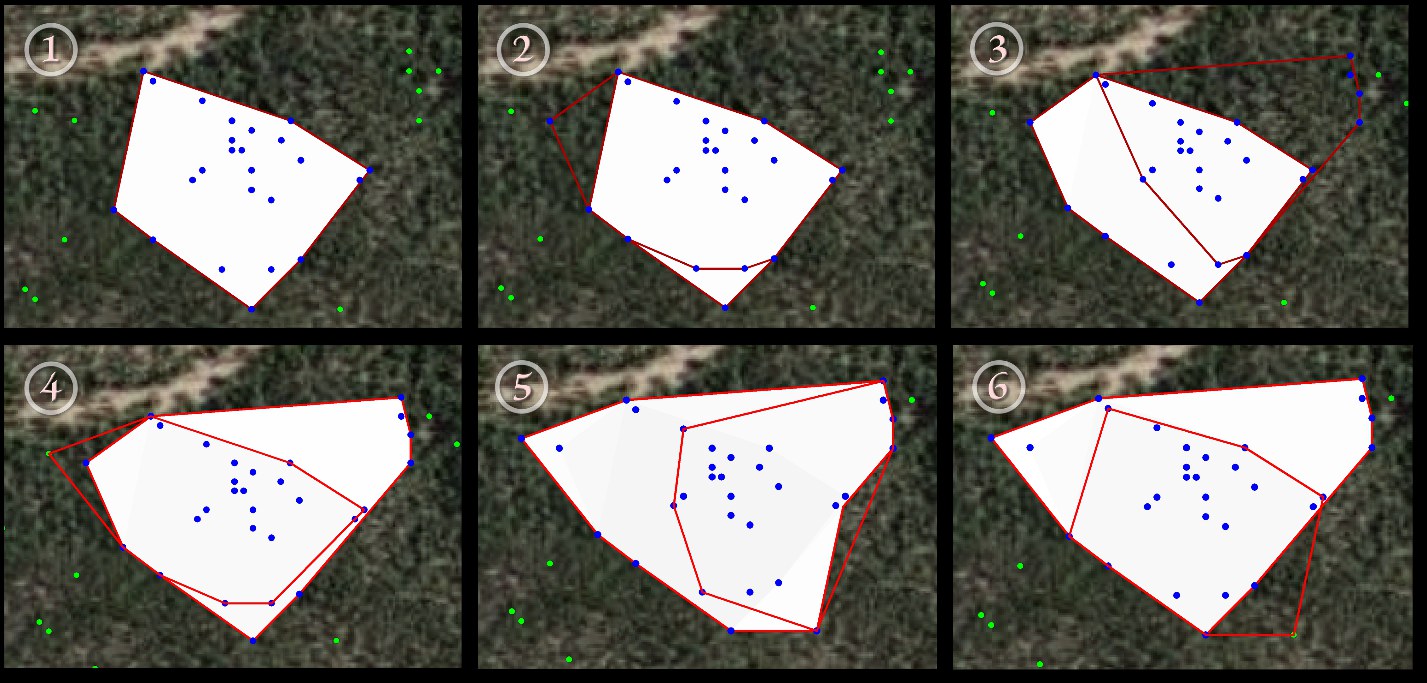
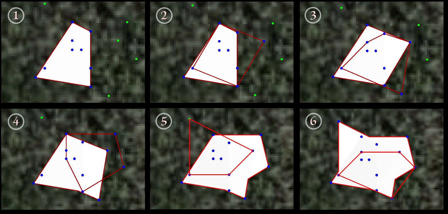
Then we sort the convex hull polygons by size, from smallest to largest, and start combining them. We create a new empty feature class, add the smallest polygon to it, then dissolve the smallest polygon with the next smallest and add that; this second combined polygon covers all the ground of the two smallest hulls. Then we dissolve in the third-smallest and add that, and so on — each combined polygon covering everything the hulls so far have covered — until the last polygon covers the entire region spanned by all the hulls. The first six iterations at k = 25 look like this:
And at k = 10:
Finally we go through all the dissolved polygons and count how many points each of them intersects. The first (smallest) one contains only k points, and the last (largest) is guaranteed to contain them all — and once we have each polygon's point count, the proportion of points it covers follows immediately. This last step is what lets us identify the regions that contain some proportion of activity we care about: the region holding 90% of all activity, or the more important areas holding the innermost 10%.
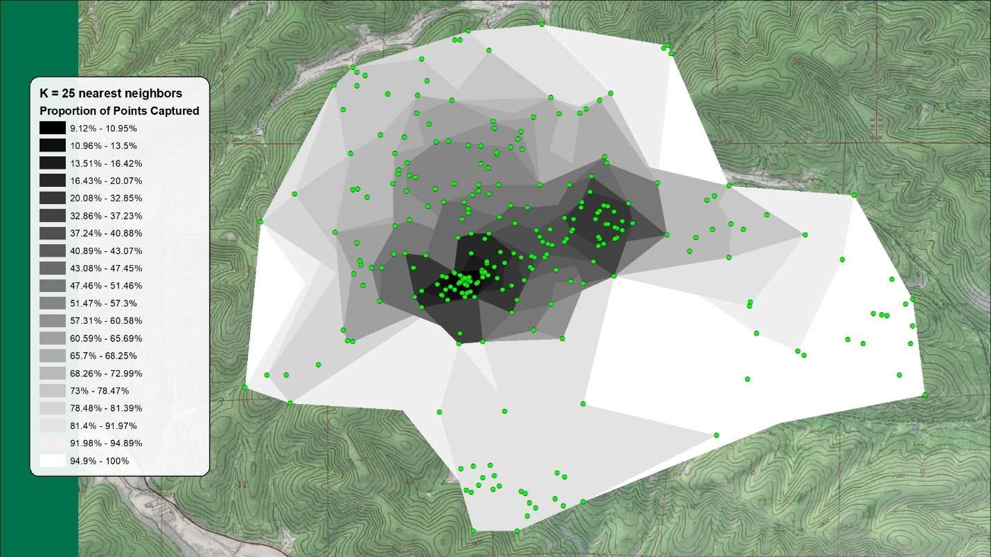
The final result at k = 25, shaded by the proportion of points captured, looks like this:
And at k = 10:
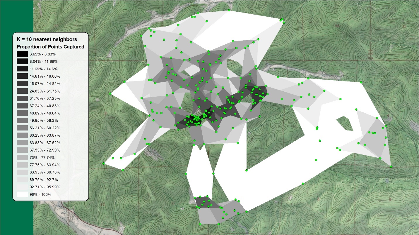
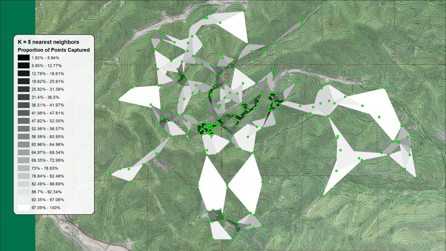
Notice how these final datasets allow for sharp boundaries at the edge of the cloud of locations, yet also allow for indents in the edge, and for holes inside the general range where the animal appears to avoid. And you can control the size of those gaps and indentations by using different values of k. At k = 5, we get a much tighter fit around the local clusters of points:
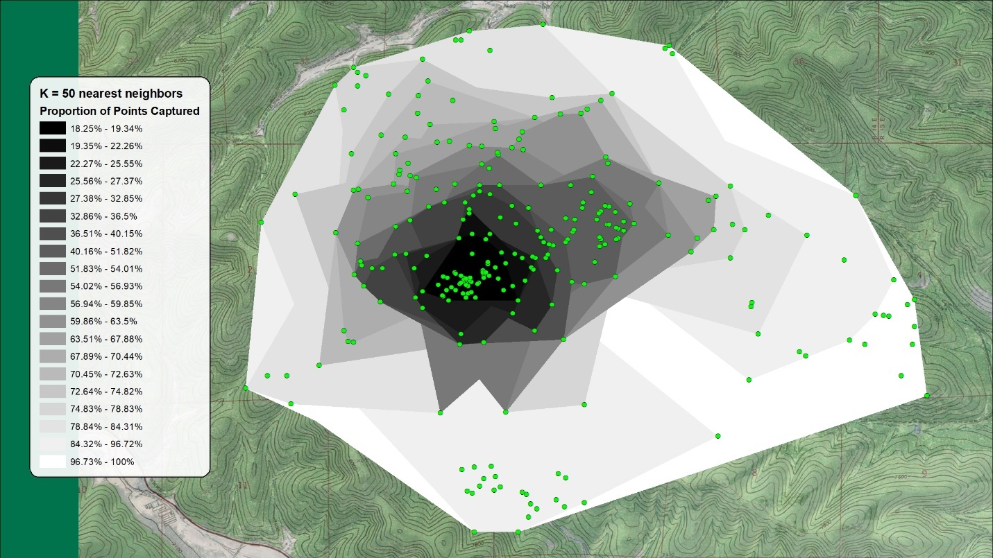
At k = 50, the overall extent is much closer to the original MCP — but we still have the advantage of seeing where activity is highest:
This walkthrough is exactly the Standard (k) variant — and the Adaptive and Fixed Sphere variants change the first step, who joins each point's hull, plus one detail of the sort. The Standard variant sorts by hull area, smallest first: every hull holds exactly k points, so a small hull is a dense hull. In the Adaptive and Fixed Sphere variants the hulls hold varying numbers of points, so they sort by point count instead, most points first (ties going to the smaller hull) — a hull that packed in many points is a dense-use hull directly. Either way the ordering means “densest first,” and everything after — the cumulative dissolve and the point proportions — is the same machine. (When this walkthrough was first written for the wildlife GIS lab, LoCoH was not in any standard toolbox and required custom code; these three tools are that code, ready-made.)
The three variants: k, a, and r
All three variants differ in exactly one decision: which points count as the focal point's neighborhood.
Standard (k-LoCoH) — the original, and exactly the method illustrated in the walkthrough above: each hull is built from the focal point and its k − 1 nearest neighbors, k points in all, and the hulls are sorted by area, smallest first (with k points in every hull, the smallest hulls are the densest). One knob, easy to reason about; hull size adapts to density automatically since the k nearest points are close in dense country and far in sparse.
Adaptive (a-LoCoH) — each focal point is given a distance budget a: neighbors are added nearest-first until their cumulative distance from the focal point reaches a. Dense neighborhoods afford many neighbors on the budget, sparse ones few — the variant that adapts most gracefully when fix density varies strongly across the range (and like the Fixed Sphere variant, at least the focal point and its two nearest neighbors are always included, so every hull can form a polygon). Because its hulls hold varying numbers of points, they are sorted by point count, most first (ties to the smaller hull), rather than by area.
Fixed Sphere (r-LoCoH) — each hull is built from all points within a sphere of influence of radius r (always including at least the focal point's two nearest neighbors, so every hull is a polygon). The neighborhood has a fixed spatial scale, which makes r the natural choice when a biologically meaningful distance — a perception range, a daily movement radius — should set the scale rather than the data's own density. Like the Adaptive variant, its hulls are sorted by point count, most first (ties to the smaller hull).
Choosing the parameter
Every variant has one governing parameter, and the same logic guides all three: small values give tight, fragmented hulls that capture fine structure and hard boundaries; large values give smooth, contiguous ranges; too small leaves spurious holes and slivers, too large inflates the range toward the MCP. Getz and Wilmers (2004) recommend the minimum spurious hole covering (MSHC) rule: choose the smallest value that fills the holes you judge spurious — the Swiss-cheese artifacts of an under-sized parameter — while the real holes, the lake the animal never swims or the cliff face it never crosses, stay open. Telling the two apart takes no prior estimate of the range's true area; it takes knowing the landscape.
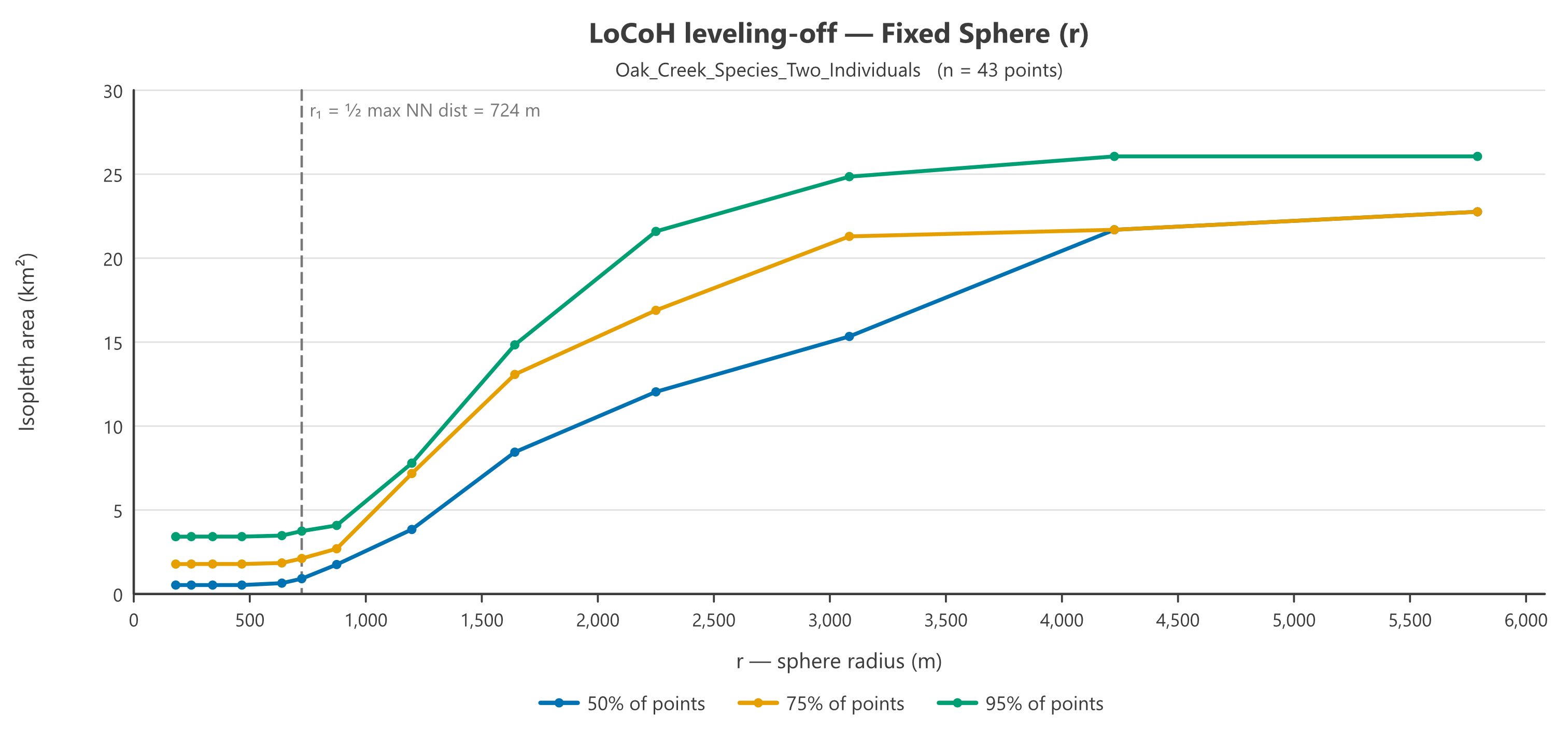
The practical procedure (Getz et al. 2007; Lyons, Turner and Getz 2013) is empirical. Build the hulls for a sequence of parameter values and plot the area enclosed by each of a family of isopleth levels — say the 10% through 95% levels, one curve per level — against the parameter. At small values the areas climb quickly as spurious holes fill in; the curves then flatten into a plateau; and past the plateau they climb again as genuinely unused ground — real holes, open bays — begins to be bridged. Choose a value on the plateau, and treat any sudden jump in a curve with suspicion: a jump is the signature of hulls suddenly spanning a gap. The T-LoCoH package (Lyons, Turner and Getz 2013) pairs the area curves with edge-to-area ratio curves for the lower (core) isopleths — spurious slivers inflate edge relative to area — and, always, with visual inspection of the isopleth maps themselves. Note that nowhere does this require knowing the true home-range area in advance: on manufactured data with known boundaries, Getz et al. could score parameter values by their Type I and Type II errors, but the field procedure reads only the shape of the curves and your own knowledge of which holes are real. Getz et al. are candid that judging when the leveling-off has been reached is a skill that comes with experience — one more reason the optional individual-hulls output is worth writing while you tune. Each variant also has a published starting heuristic — k ≈ √n; a = the maximum distance between any pair of points (typically within 30% of optimal in Getz et al.'s trials); r = half the maximum nearest-neighbor distance — described on each tool's page.
All of this sweeping and plotting is built into the LoCoH Parameter Explorer window: pick the points, pick the variant, and it draws the leveling-off curves for you, heuristic marked. The example below sweeps the radius of the Fixed Sphere variant over the two-individual Oak Creek dataset — two clusters of locations with a gap between them:
One caution applies to the whole family: LoCoH is sensitive to outliers. A bad fix far from the range still gets a hull, and its neighbors stretch to reach it. Screen out obvious location errors before running.
What the tools produce
Each tool's primary output is the dissolved cumulative isopleths: one polygon feature class in which every feature records its area, the number of locations it encloses (Point_Count), and the proportion of all locations (Point_Proportion) — select the feature nearest 0.95 and you are holding the conventional home range. An optional second output holds the individual local hulls with their own areas, point counts and densities, the raw material of the estimate and the thing to inspect when tuning the parameter. Geographic (latitude–longitude) inputs are handled with Haversine distances and WGS84 spheroidal areas; projected inputs use planar measures in the input coordinate system. The tools honor the Output Coordinate System environment for the final polygons.
References
- Getz, W. M., and C. C. Wilmers. 2004. A local nearest-neighbor convex-hull construction of home ranges and utilization distributions. Ecography 27:489–505. doi.org/10.1111/j.0906-7590.2004.03835.x
- Getz, W. M., S. Fortmann-Roe, P. C. Cross, A. J. Lyons, S. J. Ryan, and C. C. Wilmers. 2007. LoCoH: nonparametric kernel methods for constructing home ranges and utilization distributions. PLoS ONE 2(2):e207. doi.org/10.1371/journal.pone.0000207
- Lyons, A. J., W. C. Turner, and W. M. Getz. 2013. Home range plus: a space-time characterization of movement over real landscapes. Movement Ecology 1:2. doi.org/10.1186/2051-3933-1-2
Related tools and pages
- LoCoH (Standard), LoCoH (Adaptive), and LoCoH (Fixed Sphere) — the three tools this page underpins.
- Concave Hull — a single footprint polygon for a point cloud, when the question is the outline rather than the utilization distribution.
- LoCoH Parameter Explorer — sweep the parameter and chart the leveling-off curves before committing to a value.
- The Enhanced Kernel Density tools — the smooth-surface alternative, with contour and proportion companions.