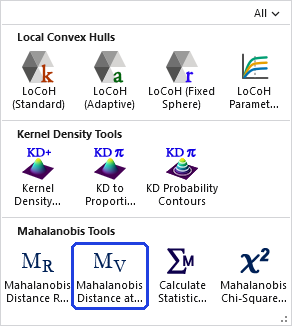
Mahalanobis Distance at Points

Home Range · geoprocessing tool · by Jeff Jenness

Works at every ArcGIS Pro license level

Learn more About Mahalanobis distances covers the theory — what the distances measure, a worked example, the chi-square p-value transform, and how the four Mahalanobis tools fit together.

Summary

Calculates a Mahalanobis value at each input point, measuring how far the point's combination of landscape-variable values lies from a multivariate reference mean, scaled by the inverse covariance among the variables. Where the Raster tool answers “how similar is every cell?”, this one answers “how typical is each of these locations?” — useful for scoring new observations against an established reference sample, or for flagging multivariate outliers within a sample.

How it works

Each point's value is the same quadratic form D² = (x − μ)′ Σ⁻¹ (x − μ) that the Mahalanobis Distance Raster tool maps, with x the vector of landscape-variable values sampled at the point. The output is a copy of the input points — all the original attribute fields are preserved — with one added DOUBLE field per selected output value:

Field	Value
Mahal_D2	The squared distance — the traditional ecological-modeling quantity.
Mahal_D	The distance (square root of D²).
Mahal_pval	The chi-square p-value: a 0 to 1 similarity score, values near 1 indicating a point that closely matches the reference conditions (df = number of variables; see the degrees-of-freedom note).

Check at least one. A point that falls outside the extent of any landscape raster, or on a NoData cell, receives a null value (−999 in a shapefile, which cannot store nulls).

Variables and statistics

The landscape variables are specified exactly as in the other Mahalanobis tools: rasters (cell values only; multiband rasters expand to one variable per band, with a Bands to exclude table) plus optional polygon variables rasterized from a numeric field — and the same order matters warning applies when reusing saved statistics.

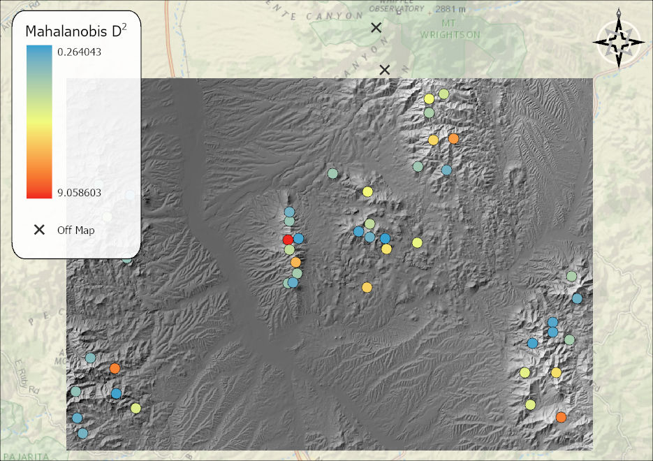
The reference mean and covariance can be computed from a point sample or read from saved tables. The point sample defaults to the input points themselves — the common case. Keep in mind that these are statistical distances, not distances across the landscape: each point is scored by how unusual its combination of variable values (its elevation, slope, and so on) is compared with the average conditions over all the points. A point can sit in the geographic middle of the cluster and still score as a strong outlier if it happens to fall on an odd patch of ground — and that is exactly how you spot the outliers.

Alternatively, supply a separate statistics layer to score the input points against a different reference sample. You might score candidate survey sites against conditions at verified nest sites, this year's telemetry locations against last year's established sample, or one animal's locations against another's. If you are wondering how the two point layers get connected to each other — they don't, and they don't need to. The statistics points are used once, up front, to define the reference conditions: the landscape variables are sampled at their locations to build the mean vector and covariance matrix, and then those points exit the stage. Each input point is scored by sampling the same variables at its location and comparing that combination of values against the reference statistics. The two layers connect only through the shared landscape variables, never point-to-point. (Supplying a statistics layer here is exactly equivalent to running Calculate Statistical Matrices on it first and choosing Existing tables.)

With Existing tables, the mean and covariance come from tables saved earlier by Calculate Statistical Matrices or the Raster tool, with the variable order validated.

The Cell value sampling choice (exact vs. bilinear) and the Covariance inversion method (standard vs. SVD pseudo-inverse, with the condition number reported) behave as described on the Raster page. The same four optional statistics tables (mean, covariance, inverse covariance, correlation) can be saved for reuse.

Environments

The tool honors the Output Coordinate System, Cell Size, Processing Extent, and Snap Raster environments — they define the grid on which the landscape variables are sampled. Other geoprocessing environments do not affect it.

A tour of the dialog

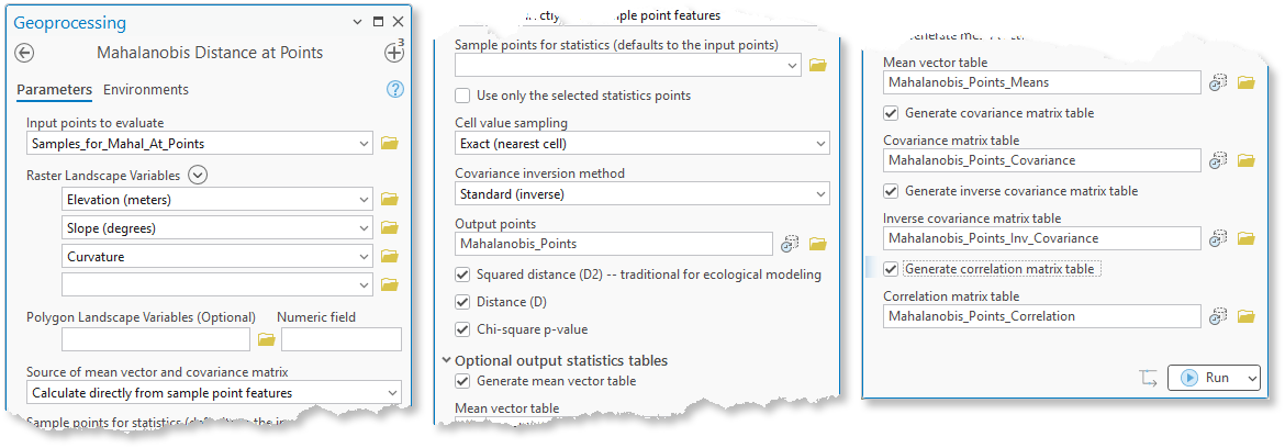
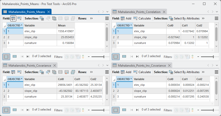
Here the tool evaluates a set of sample points against elevation, slope and curvature, with the statistics computed from the input points themselves and all three output values requested. Notice that this example also generates all four statistical tables — the checkboxes toward the bottom of the pane write the mean vector, covariance, inverse covariance and correlation matrices alongside the scored points:

The Home Range Tools gallery open on the ribbon, with the Mahalanobis Distance at Points button, in the Mahalanobis Tools row, outlined in blue — Where to find it: **Mahalanobis Distance at Points** is in the *Mahalanobis Tools* row of the *Home Range Tools* gallery, in the Home Range group of the *Wildlife and Forestry* tab.

The Mahalanobis Distance at Points pane in three panels: elevation, slope and curvature as raster variables with statistics calculated directly from sample point features; the statistics-points override left empty with exact cell sampling; and all three output value checkboxes checked with the four optional statistics tables enabled — The dialog, top to bottom: the input points and landscape variables; the statistics source (the statistics-points override left empty, so the input points themselves supply the statistics); the three output-value checkboxes; and the optional statistics tables.

The output points over a hillshaded landscape, colored by their Mahalanobis D-squared values from blue for low through yellow to red for high, with two points beyond the northern edge of the landscape rasters drawn as X markers labeled Off Map — The output points, symbolized by their **Mahal_D2** field: blue points sit on terrain typical of the sample as a whole; the red and orange points are the multivariate outliers. Notice the two X markers at the top — those points fell outside the landscape rasters, were skipped (with a warning in the run messages), and carry *null* values, so they can be symbolized — or excluded — deliberately.

The four optional output tables open in ArcGIS Pro: the mean vector with one row per variable, and the covariance, inverse covariance and correlation matrices, each row labeled by variable name — The four optional statistics tables. Each row is labeled by variable, in the analysis order — the mean and covariance pair can feed later runs through the Existing-tables source, and the correlation matrix is the place to screen for collinear variables.

ModelBuilder

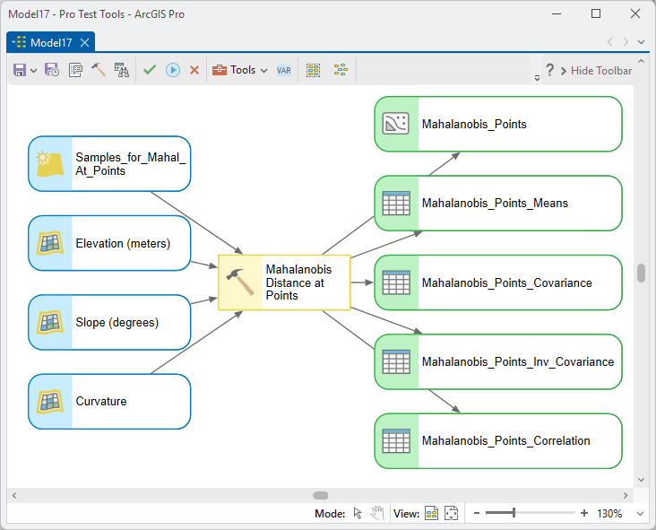
The output feature class is the model output; downstream tools can select on the value fields (for example, Mahal_pval < 0.05 to pull out the atypical locations for review) or join them back to the source data.

Parameters

Label	Explanation	Data type
Input points to evaluateRequired · target_points	The point features at which to compute the Mahalanobis values. Each feature gets one value, so these must be single points, not multipoints.	Feature Layer
Raster Landscape VariablesRequired · raster_vars	The rasters defining the multivariate space; at least one is required and sets the analysis grid.	Raster Layer (multiple)
Polygon Landscape VariablesOptional · poly_vars	Polygon feature class + numeric field rows, rasterized to the analysis grid.	Value Table
Bands to excludeOptional · exclude_bands	Multiband raster + 1-based band number rows to drop.	Value Table
Source of mean vector and covariance matrixRequired · stats_source	A point sample, or existing tables; choose the source first and the relevant inputs below enable accordingly.	String
Sample points for statistics (defaults to the input points)Optional · stats_points	Leave empty to use the input points themselves (the common case).	Feature Layer
Use only the selected statistics pointsOptional · use_selected	Restrict the statistics to the layer's active selection.	Boolean
Mean vector tableOptional · mean_table	A saved mean vector (existing-tables source only).	Table View
Covariance matrix tableOptional · cov_table	A saved covariance matrix; its stored variable order validates the variable list.	Table View
Cell value samplingOptional · sample_method	Exact (nearest cell) or Interpolated (bilinear).	String
Covariance inversion methodRequired · inversion	Standard (inverse) or Pseudo-inverse (SVD).	String
Output pointsRequired · out_points	Copy of the input points (all original attribute fields preserved) with the value fields added; defaults to Mahalanobis_Points, auto-incremented.	Feature Class
Squared distance (D²) / Distance (D) / Chi-square p-valueOptional · out_d2, out_d, out_pval	Which value fields to write (Mahal_D2, Mahal_D, Mahal_pval); at least one must be checked.	Boolean
Generate / save statistics tablesOptional · gen_mean…save_corr	Checkbox-and-output pairs for the mean vector, covariance, inverse covariance, and correlation tables.	Boolean + Table

Python

D² and p-value at each observed location, statistics from those same points:

import arcpy
arcpy.ImportToolbox(r"C:\path\to\JennessEnterprisesTools.pyt")  # your install path
arcpy.jenness.MahalanobisPoints(
    target_points="Observed_Locations",
    raster_vars="elev_clip;slope_clip;curvature",
    sample_method="Interpolated (bilinear)",
    stats_source="Calculate directly from sample point features",
    inversion="Standard (inverse)",
    out_points=r"C:\Project\Mahalanobis.gdb\Observed_Mahal",
    out_d2=True,
    out_d=False,
    out_pval=True)

Recommended citation

Jenness, J. 2026. Mahalanobis Distance at Points. Wildlife and Forestry Tools add-in for ArcGIS Pro, v. 1.99 (September 2026). Jenness Enterprises. Available at: https://github.com/JeffJenness/Wildlife_Tools.

Credits and references

By Jeff Jenness, Jenness Enterprises (www.jennessent.com), ported from his ArcView Mahalanobis Distances extension and the ArcMap Land Facet Corridor Tools.

Clark, J. D., J. E. Dunn, and K. G. Smith. 1993. A multivariate model of female black bear habitat use for a geographic information system. Journal of Wildlife Management 57:519–526. doi.org/10.2307/3809276
Farber, O., and R. Kadmon. 2003. Assessment of alternative approaches for bioclimatic modeling with special emphasis on the Mahalanobis distance. Ecological Modelling 160:115–130. doi.org/10.1016/S0304-3800(02)00327-7
Mahalanobis, P. C. 1936. On the generalised distance in statistics. Proceedings of the National Institute of Sciences of India 2(1):49–55. Reprinted 2018 in Sankhyā A 80(Suppl 1):S1–S7. doi.org/10.1007/s13171-019-00164-5

Licensing information

Works at every ArcGIS Pro license level (Basic, Standard, Advanced). No extension licenses are required.

About Mahalanobis distances — theory, worked example, and the chi-square p-value discussion.
Mahalanobis Distance Raster — the same value for every cell of the landscape.
Calculate Statistical Matrices — compute the reference statistics once, reuse them here.
Mahalanobis Chi-Square Transform — the raster-side p-value rescaling.

Mahalanobis Distance at Points

Summary

How it works

Variables and statistics

Environments

A tour of the dialog

ModelBuilder

Parameters

Python

Recommended citation

Credits and references

Licensing information

Related tools and pages