

Calculate Statistical Matrices
Summary
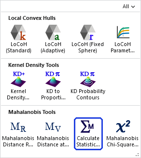
Computes the mean vector, covariance matrix, inverse covariance matrix, and/or correlation matrix for a set of landscape variables and writes them as tables. This is the producer tool of the Mahalanobis suite: compute the statistics once from your best reference sample, then supply the mean and covariance tables to Mahalanobis Distance Raster or at Points through their Existing tables source — the statistics aren't recomputed for every run, and every run is guaranteed to use exactly the same reference.
What it computes
The Mahalanobis formula D² = (x − μ)′ Σ⁻¹ (x − μ) needs two ingredients: the mean vector μ and the covariance matrix Σ. This tool derives both, either from sample point features (the landscape variables sampled at the points, optionally only the selected ones) or from the cells of a categorical raster matching a chosen category. Categories can be picked by any field of the raster's attribute table — choose Landfire's broad EVT_LF = “Tree” and every tree-type cell value joins the sample automatically — or by the literal cell value when there is no attribute table (the fuller discussion is on the Raster page). The landscape variables are specified exactly as in the other Mahalanobis tools — rasters (multiband rasters expand to one variable per band), plus optional polygon variables rasterized from a numeric field.
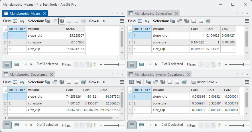
Two further tables are optional extras for inspection rather than reuse: the inverse covariance (computed by your chosen inversion method — the consuming tools invert the covariance themselves, so this table is never required) and the correlation matrix, the natural place to screen for collinear variables before they cause trouble. A pair of strongly correlated variables contributes little independent information and pushes the covariance toward singularity — the tool reports the covariance condition number, and very large values are the warning sign.
Environments
The tool honors the Output Coordinate System, Cell Size, Processing Extent, Snap Raster, and Mask environments when aligning the landscape variables to a common analysis grid. Other geoprocessing environments do not affect it.
A tour of the dialog
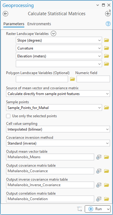
Here the statistics are computed from a sample-point layer over three landscape variables — slope, curvature and elevation, in that order — with all four output tables requested:
ModelBuilder
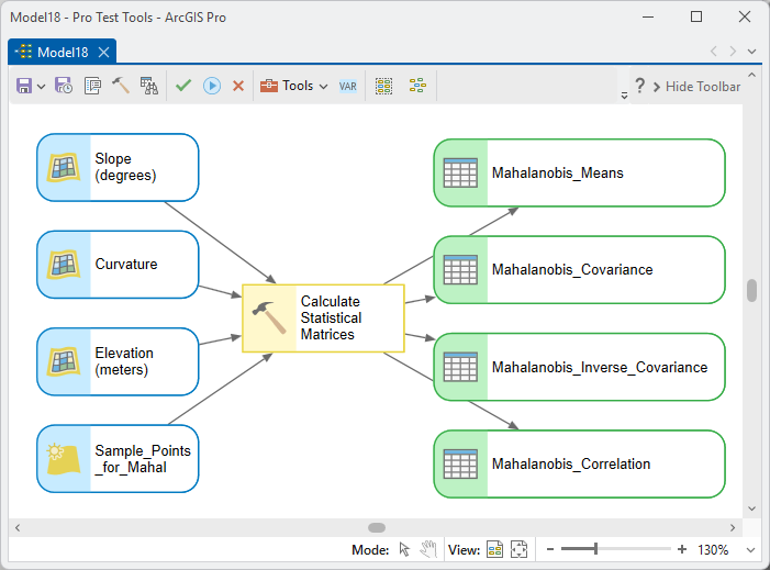
All four tables are model outputs. The natural pattern: compute the mean and covariance once at the head of a model, then fan those two tables out to several Mahalanobis Raster or at Points runs — different landscapes, years, or study areas, all scored against the identical reference.
Parameters
| Label | Explanation | Data type |
|---|---|---|
| Raster Landscape VariablesRequired · raster_vars | The rasters defining the multivariate space; at least one is required and sets the analysis grid. | Raster Layer (multiple) |
| Polygon Landscape VariablesOptional · poly_vars | Polygon feature class + numeric field rows, rasterized to the analysis grid. | Value Table |
| Bands to excludeOptional · exclude_bands | Multiband raster + 1-based band number rows to drop. | Value Table |
| Source of mean vector and covariance matrixRequired · stats_source | Sample point features or categorical raster; choose the source first and the relevant inputs below enable accordingly. (The Existing-tables option is intentionally absent here — this tool produces those tables.) | String |
| Sample pointsOptional · points | The reference points; points outside the landscape data or on NoData cells are excluded and reported. | Feature Layer |
| Use only the selected pointsOptional · use_selected | Restrict the statistics to the layer's active selection. | Boolean |
| Categorical rasterOptional · cat_raster | The raster whose matching cells form the reference sample. | Raster Layer |
| Category attribute fieldOptional · cat_field | A field from the raster's attribute table naming the categories the way you want to choose them; leave blank to enter a literal cell value instead. | Field |
| Category valueOptional · cat_value | The category whose cells form the reference sample — a dropdown of the chosen field's values, with every matching cell value gathered automatically. With no field, literal cell value(s), semicolon-separated for several (“3;4;5”). | String |
| Cell value samplingOptional · sample_method | Exact (nearest cell) or Interpolated (bilinear); bilinear suits continuous surfaces, exact suits categorical rasters. | String |
| Covariance inversion methodRequired · inversion | Standard (inverse) or Pseudo-inverse (SVD); used only when the inverse covariance table is requested. | String |
| Output mean vector tableOptional · out_mean | The mean vector (one row per variable), auto-named Mahalanobis_Means; clear to skip. | Table |
| Output covariance matrix tableOptional · out_cov | The covariance matrix, auto-named Mahalanobis_Covariance; clear to skip. Together with the mean vector, this is what the consuming tools read. | Table |
| Output inverse covariance matrix tableOptional · out_invcov | For inspection; never required for reuse. | Table |
| Output correlation matrix tableOptional · out_corr | For screening collinearity among the variables. | Table |
Python
Mean and covariance from three rasters sampled at a point layer, with the two optional inspection tables:
import arcpy
arcpy.ImportToolbox(r"C:\path\to\JennessEnterprisesTools.pyt")  # your install path
out_gdb = r"C:\Project\Mahalanobis.gdb"
arcpy.jenness.MahalanobisCovariance(
    raster_vars="elev_clip;slope_clip;curvature",
    sample_method="Interpolated (bilinear)",
    stats_source="Calculate directly from sample point features",
    points="Sample_Points_for_Mahal",
    inversion="Standard (inverse)",
    out_mean=out_gdb + r"\Mahalanobis_Means",
    out_cov=out_gdb + r"\Mahalanobis_Covariance",
    out_invcov=out_gdb + r"\Mahalanobis_Inv_Covariance",
    out_corr=out_gdb + r"\Mahalanobis_Correlation")
For categorical-raster statistics, pass the attribute field
and category value exactly as in the dialog
(stats_source="Categorical raster", cat_raster="Landfire",
cat_field="EVT_LF", cat_value="Tree") — the tool
gathers the matching cell values itself. Or skip the field and
give literal cell value(s), semicolon-separated for several
(cat_field=None, cat_value="7016;7019;7023"); the
full example is on the
Raster
page.
Recommended citation
Credits and references
By Jeff Jenness, Jenness Enterprises (www.jennessent.com), ported from his ArcView Mahalanobis Distances extension and the ArcMap Land Facet Corridor Tools.
- Clark, J. D., J. E. Dunn, and K. G. Smith. 1993. A multivariate model of female black bear habitat use for a geographic information system. Journal of Wildlife Management 57:519–526. doi.org/10.2307/3809276
- Mahalanobis, P. C. 1936. On the generalised distance in statistics. Proceedings of the National Institute of Sciences of India 2(1):49–55. Reprinted 2018 in Sankhyā A 80(Suppl 1):S1–S7. doi.org/10.1007/s13171-019-00164-5
Licensing information
Works at every ArcGIS Pro license level (Basic, Standard, Advanced). No extension licenses are required.
Related tools and pages
- About Mahalanobis distances — what the mean vector and covariance matrix do in the formula.
- Mahalanobis Distance Raster and Mahalanobis Distance at Points — the consumers of these tables, through their Existing-tables source.
- Mahalanobis Chi-Square Transform — the final step from D² to a typicality surface.