

Local Convex Hull (LoCoH) — Adaptive
Summary
Estimates an animal's home range and utilization distribution by the Adaptive (a-) Local Convex Hull method of Getz et al. (2007): every location is given a distance budget a, and its neighbors are added nearest-first until their cumulative distance from the focal point reaches the budget. The hulls are sorted by point count, most points first (ties going to the smaller hull), and merged cumulatively into density isopleths. Outputs are the dissolved cumulative isopleths — each carrying the adaptive cumulative distance alongside its area and point statistics — and, optionally, the individual hulls.
How the distance budget shapes the hulls
Where the Standard variant counts neighbors, the Adaptive variant spends distance. Each focal point sorts the other locations by distance and adds them, nearest first, until their cumulative distance reaches a. In dense country the nearest neighbors are cheap, so the budget affords many of them; in sparse country each neighbor is expensive and the budget buys few. That is the variant's strength: when fix density varies strongly across a range — a heavily-used core plus lightly-sampled excursion country — the neighborhoods adapt themselves, and Getz et al. (2007) found the a-method the most robust of the three in such conditions. Larger a gives larger, smoother hulls; smaller a gives tighter, more fragmented ones — and at least the focal point and its two nearest neighbors are always included, whatever the budget, so every hull forms a polygon.
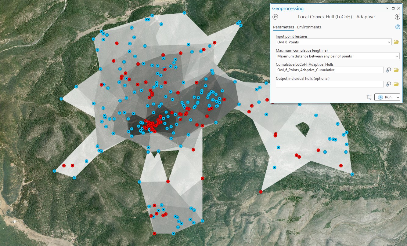
Choosing a. Getz et al. (2007) suggest starting with a equal to the maximum distance between any pair of points — the tool's automatic option — then refining downward by the minimum spurious hole covering rule, watching isopleth areas across a range of values as the T-LoCoH package recommends (Lyons, Turner and Getz 2013). The LoCoH Parameter Explorer window automates that refinement: it sweeps the budget from very small values up to a₁ and draws the leveling-off curves, so you can read the stable zone straight off the chart before running this tool. When you specify the length yourself it may be entered in any linear unit; it is converted to meters internally, and the adaptive cumulative distance is reported in the unit you chose. Screen out obvious location errors first; LoCoH is sensitive to outliers.
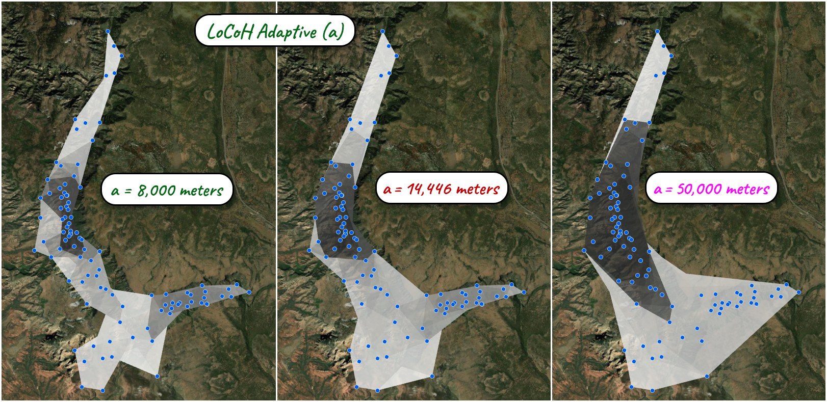
What you get
The primary output holds the dissolved cumulative isopleths: each feature stores its dissolved area (Area), enclosed point count (Point_Count), point proportion (Point_Proportion), the adaptive cumulative distance (Adaptive_Cumulative_Dist), and point density in points per square kilometer (Pts_per_SqKm). The optional second output holds the individual local hulls with their own areas, point counts, proportions, densities and cumulative distances. Geographic inputs use Haversine distances and WGS84 spheroidal areas; projected inputs use planar measures. Area is in square meters for geographic inputs and in square map units for projected inputs. The Output Coordinate System environment is honored for the final polygons.
A tour of the dialog
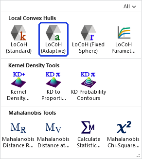
A run needs the points, a choice for the budget — the automatic maximum pairwise distance, or a length you specify — and an output name; the individual hulls are one optional output more.
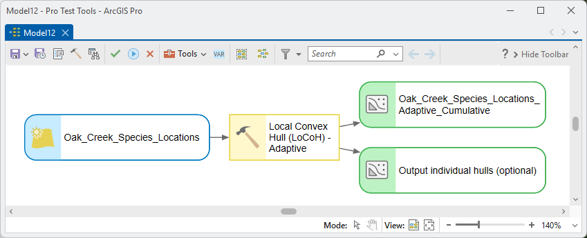
ModelBuilder
Both outputs chain onward in a model — the isopleth polygons feed clip, overlay, or reporting steps directly, and a Select on Point_Proportion pulls the 95% or 50% isopleth out of the stack for the next tool.
Parameters
| Label | Explanation | Data type |
|---|---|---|
| Input point featuresRequired · in_features | The point features (GPS or VHF telemetry fixes, for example) the local hulls are built from. Geographic or projected; empty geometries are ignored. Every point of a multipoint feature is used. | Feature Layer |
| Maximum cumulative length (a)Required · a_method | How a is determined: the maximum distance between any pair of points (the Getz et al. 2007 heuristic), or Specify a length to enter your own. | String |
| LengthOptional · a_length | The budget itself, used only with Specify a length. Any linear unit; converted to meters internally, and the adaptive distance is reported in your unit. | Linear Unit |
| Cumulative LoCoH [Adaptive] HullsRequired · out_isopleths | The dissolved cumulative isopleths, each with Area, Point_Count, Point_Proportion, Adaptive_Cumulative_Dist, and Pts_per_SqKm. | Feature Class |
| Output individual hulls (optional)Optional · out_hulls | The individual local convex hulls, each with its own area, point count, proportion, cumulative distance and density. | Feature Class |
Python
An adaptive LoCoH using the automatic maximum pairwise distance, with both outputs:
import arcpy
arcpy.ImportToolbox(r"C:\path\to\JennessEnterprisesTools.pyt")  # your install path
arcpy.jenness.LoCoHAdaptive(
    in_features=r"D:\data\telemetry.gdb\owl_fixes",
    a_method="Maximum distance between any pair of points",
    out_isopleths=r"D:\data\telemetry.gdb\owl_isopleths_a",
    out_hulls=r"D:\data\telemetry.gdb\owl_hulls_a")
Recommended citation
Credits and references
By Jeff Jenness, Jenness Enterprises (www.jennessent.com), implementing the a-LoCoH method of Getz and colleagues. Full references on the About LoCoH page.
- Getz, W. M., S. Fortmann-Roe, P. C. Cross, A. J. Lyons, S. J. Ryan, and C. C. Wilmers. 2007. LoCoH: nonparametric kernel methods for constructing home ranges and utilization distributions. PLoS ONE 2(2):e207. doi.org/10.1371/journal.pone.0000207
- Lyons, A. J., W. C. Turner, and W. M. Getz. 2013. Home range plus: a space-time characterization of movement over real landscapes. Movement Ecology 1:2. doi.org/10.1186/2051-3933-1-2
Licensing information
Works at every ArcGIS Pro license level (Basic, Standard, Advanced). No extension licenses are required.
Related tools and pages
- About LoCoH home-range analysis — the shared theory.
- LoCoH (Standard) — a fixed neighbor count; the original, and the easiest knob to reason about.
- LoCoH (Fixed Sphere) — a fixed radius, when a biologically meaningful distance should set the scale.
- LoCoH Parameter Explorer — sweep the parameter and chart the leveling-off curves before committing to a value.
- Concave Hull — one clean footprint polygon instead of a utilization distribution.